---
title: "Generative Models"
format:
html:
code-fold: true
toc: true
theme: cosmo
jupyter: python3
filters:
- shinylive
---
Every model in this course so far has taken a molecule as input, whether to predict a property from it or, as in the [unsupervised methods](11_unsupervised_learning.qmd) of the previous chapter, to find structure in a set of them. The molecules themselves always came from outside, from a database or a screening library.
**Generative models** instead produce new molecules and make *inverse design* possible.
The chapter begins with **genetic algorithms**, which predate deep learning and remain a strong baseline. It then turns to deep generative models: **variational autoencoders**, **diffusion models**, and the **generative language models** that build on the [language models](09_language_models.qmd) chapter.
## Predictive vs. Generative Models
A **predictive** (or *discriminative*) model learns a conditional distribution $p(y \mid x)$: given a molecule $x$, it predicts a value of a property $y$. Regression and classification on molecular descriptors, fingerprints or graphs all fall into this category.
A **generative** model instead learns the distribution $p(x)$ of the data itself, so that new points $\tilde{x} \sim p(x)$ can be **sampled** that resemble the training set. This requires only *examples* of the data, and for unconditional generation no labels at all.
The same idea underlies familiar tools for text (ChatGPT, Claude, Gemini), images (Stable Diffusion, Midjourney) and audio (ElevenLabs, Suno). In contrast to these applications, the question of which representation (recall the [cheminformatics](02_cheminformatics.qmd) chapter) serves generative modelling best remains open for molecules.
## Conditional and Unconditional Generation
Generation comes in two forms. **Unconditional generation** produces samples resembling the training set with no further objective. **Conditional generation** produces samples conditioned on some input, such as a text prompt, a scaffold to be kept fixed, a fragment to grow, or a target property value.
**REINVENT 4** [@loeffler2024reinvent] illustrates the range with four generators:
- **Reinvent** — fully *de novo*, unconstrained: sample new molecules.
- **Mol2Mol** — molecule optimization: transform a molecule into a related, improved one.
- **Libinvent** — library design and scaffold decoration: the output depends on a provided core.
- **Linkinvent** — fragment linking and scaffold hopping: the model is primed with fragments to connect.
Conditioning is also what a chatbot does. Prompting ChatGPT to complete the partial SMILES `c1ccc` returns benzene, `c1ccccc1`; the generated text is conditioned on the prompt.
### Inverse design
A central motivation for generative models can be understood as **inverse design** [@sanchezlengeling2018inverse]. Two directions explain the name:
$$f(\mathbf{x}) = \mathbf{y} \qquad \text{vs.} \qquad \mathbf{x} = f^{-1}(\mathbf{y}).$$
**Direct design** is $f(\mathbf{x}) = \mathbf{y}$: pick molecules, obtain their properties by experiment or simulation, and keep whichever turned out best. This is brute-force screening. **Inverse design** is $\mathbf{x} = f^{-1}(\mathbf{y})$: start from the desired properties and find molecules that have them.
The second expression is optimistic, because $f^{-1}$ is not a function. Many molecules share any given property value, so the inverse is one-to-many and the realistic goal is to produce *some* molecule(s) with the target properties.
@fig-inverse-design contrasts the two, with a **functional space** of desired properties on the left and **chemical space** on the right. Direct design walks from chemical to functional space and then screens; inverse design walks the other way.
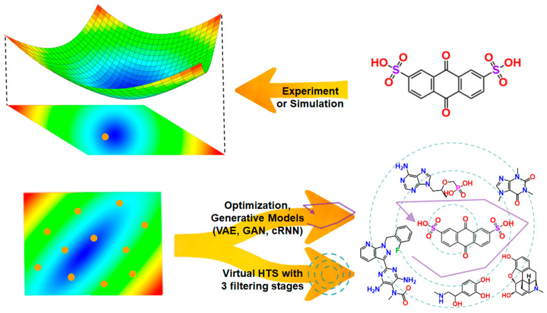{#fig-inverse-design width=85%}
Two broad strategies exist for doing this. The first searches directly over molecules, holding an explicit set of candidates and improving it. The second learns a distribution over molecules and samples from it. The chapter covers them in that order.
## Classical Generative Models
### Genetic algorithms
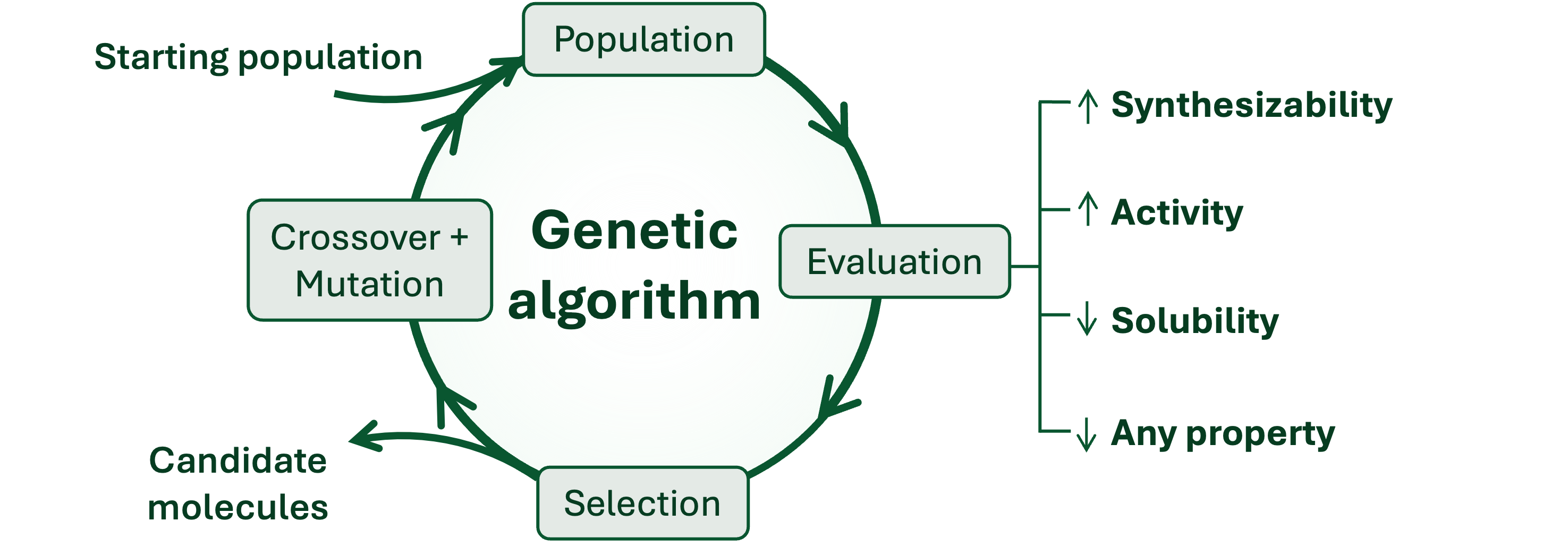
A **genetic algorithm** applies survival of the fittest to molecules over many generations. It repeats a simple loop:
1. **Population** — start from a population of $n$ molecules.
2. **Fitness calculation** — score each molecule with a machine learning model or a simulation.
3. **Selection** — remove molecules with low fitness.
4. **Crossover and mutation** — recombine and perturb highly scored molecules to create new candidates.
Over successive generations the population drifts toward higher fitness. Two properties make genetic algorithms attractive. They need no training data of their own, since a starting population and a scoring function suffice, though that scoring function is frequently a trained model itself. And they are simple yet effective: on standard benchmarks a well-tuned genetic algorithm still matches or outperforms far more elaborate deep generative models [@tripp2023gabaselines]. The scoring function requires special care, because generated molecules are only ever as good as the function used to rank them.
{#fig-ga-cycle width=90%}
The graph-based genetic algorithm of @jensen2019gb defines both crossover and mutation operations on the molecular graph. **Mutation** applies one of a fixed set of edits chosen at random with hand-tuned probabilities: appending, inserting or deleting an atom, changing a bond order or an atom type, and adding or deleting a ring bond. **Crossover** cuts two parents and rejoins the fragments, which can yield children that violate valence rules, so further rules discard them. The operations work well in practice, but every one had to be written by hand, and the authors describe the filtering rules as arbitrary.
A genetic algorithm has neither a model of the property landscape nor a gradient to follow. Its population is the only record of what has been tried and the only material from which the next generation can be built. Its behaviour is therefore a balance between **exploration**, searching widely across chemical space, and **exploitation**, refining molecules that already score well. Exploitation might miss better candidates in other regions of chemical space and produces less diverse candidates while exploration costs computational resources with rather lower chance of finding well performing structures per evaluation. Where the balance falls is set by the population size, the rate and size of mutations, and how much crossover is used relative to mutation.
The widget below runs a genetic algorithm on a two-dimensional landscape, where the axes stand in for chemical space and the surface for fitness. The population starts on a low hill, with a higher peak some distance away.
```{shinylive-python}
#| standalone: true
#| viewerHeight: 700
from shiny import App, render, ui
import matplotlib
import matplotlib.pyplot as plt
import numpy as np
matplotlib.rcParams.update({
"font.family": "serif",
"figure.facecolor": "#fafaf7",
"axes.facecolor": "#fafaf7",
"axes.grid": True,
"grid.alpha": 0.3,
})
BLUE = "#2b6cb0"
RED = "#c53030"
GREEN = "#276749"
GENS = 40
def fitness(P):
"""Two overlapping peaks: a lower one where the population starts, a higher one beyond."""
d1 = (P[:, 0] + 2.2) ** 2 + (P[:, 1] + 2.0) ** 2
d2 = (P[:, 0] - 0.8) ** 2 + (P[:, 1] - 1.0) ** 2
return np.exp(-d1 / (2 * 1.6 ** 2)) + 1.7 * np.exp(-d2 / (2 * 2.0 ** 2))
g = np.linspace(-5, 5, 140)
GX, GY = np.meshgrid(g, g)
Z = fitness(np.column_stack([GX.ravel(), GY.ravel()])).reshape(GX.shape)
def diversity(P):
d = np.linalg.norm(P[:, None, :] - P[None, :, :], axis=-1)
n = len(P)
return d.sum() / max(1, n * (n - 1))
def run(n, p_mut, mut_size, p_cross, seed):
"""Recompute the whole run from the seed so the display is reproducible."""
rng = np.random.default_rng(seed)
P = np.array([-2.2, -2.0]) + rng.normal(0, 0.5, size=(n, 2))
history = [P.copy()]
for _ in range(GENS):
parents = P[np.argsort(fitness(P))[::-1][: max(2, n // 2)]]
kids = np.empty_like(P)
for i in range(n):
a = parents[rng.integers(len(parents))]
if rng.random() < p_cross:
b = parents[rng.integers(len(parents))]
w = rng.random()
kids[i] = w * a + (1 - w) * b # a blend of two parents, never outside them
else:
kids[i] = a
if rng.random() < p_mut:
kids[i] = kids[i] + rng.normal(0, mut_size, 2)
P = kids
history.append(P.copy())
return history
app_ui = ui.page_fluid(
ui.layout_columns(
ui.input_slider("gen", "Generation", min=0, max=GENS, value=0, step=1),
ui.input_slider("mut", "Mutation size", min=0.0, max=1.0, value=0.0, step=0.05),
ui.input_slider("p_mut", "Mutation rate", min=0.0, max=1.0, value=0.3, step=0.05),
ui.input_slider("p_cross", "Crossover fraction",
min=0.0, max=1.0, value=0.8, step=0.05),
ui.input_select("n", "Population size",
choices=["6", "12", "30", "60"], selected="30"),
ui.input_slider("seed", "Random seed", min=0, max=5, value=0, step=1),
col_widths=(4, 4, 4, 4, 4, 4),
),
ui.output_plot("ga_plot"),
)
def server(input, output, session):
@render.plot
def ga_plot():
n = int(input.n())
gen = int(input.gen())
hist = run(n, float(input.p_mut()), float(input.mut()),
float(input.p_cross()), int(input.seed()))
best = np.maximum.accumulate([fitness(P).max() for P in hist])
div = [diversity(P) for P in hist]
P = hist[gen]
# constrained layout, so the axis labels survive being resized by the browser
fig, (ax, ax2) = plt.subplots(1, 2, figsize=(8.2, 3.5), layout="constrained",
gridspec_kw={"width_ratios": [1, 1]})
ax.contourf(GX, GY, Z, levels=16, cmap="Greens", alpha=0.9)
ax.contour(GX, GY, Z, levels=16, colors="white", linewidths=0.4)
ax.scatter(P[:, 0], P[:, 1], s=24, color=BLUE, edgecolors="white",
linewidths=0.6, zorder=4, label="population")
top = P[np.argmax(fitness(P))]
ax.plot(top[0], top[1], "*", ms=15, color=RED, markeredgecolor="white",
zorder=5, label="best so far")
ax.set_xlim(-5, 5)
ax.set_ylim(-5, 5)
ax.set_aspect("equal")
ax.set_xlabel("chemical space 1", fontsize=9)
ax.set_ylabel("chemical space 2", fontsize=9)
ax.set_title(f"generation {gen} of {GENS}", fontsize=10.5, fontweight="bold")
ax.tick_params(labelsize=8)
ax.legend(loc="lower right", fontsize=8)
ax.grid(False)
gens = np.arange(len(hist))
ax2.plot(gens, best, color=RED, lw=2.0, label="best fitness so far")
ax2.plot(gens, div, color=GREEN, lw=1.8, ls="--", label="population diversity")
ax2.axvline(gen, color="#a0aec0", lw=1.2, ls=":")
ax2.set_xlim(0, GENS)
ax2.set_ylim(0, max(2.0, max(div) * 1.1))
ax2.set_xlabel("generation", fontsize=9)
ax2.set_title("progress and diversity", fontsize=10.5, fontweight="bold")
ax2.tick_params(labelsize=8)
ax2.legend(loc="upper right", fontsize=8)
return fig
app = App(app_ui, server)
```
With the mutation size at zero the population never leaves the region it started in, however many generations are run. The crossover used here averages two parents, so offspring can only fall between them and the population collapses onto a single point: the diversity curve falls to zero and the best fitness plateaus well below the higher peak. Any non-zero mutation breaks that limit and the population climbs to the better region, with larger mutations arriving sooner but leaving the final population more scattered. The smallest population loses its diversity fastest and is the least reliable at finding the better region, which is why real runs use populations of hundreds to thousands.
Averaging is the simplest possible crossover. Graph crossover builds children that can have quite different properties than their parents span, so in a real molecular run crossover contributes to exploration too. What survives the simplification is the general point that the two operators play different roles, and that the balance between them is a setting to be tuned.
An alternative to the presented hand-coded graph operations is to operate on a string representation instead.
### SELFIES and the STONED algorithm
SMILES strings can easily be written that describe no molecule at all. `CC(C)(C)(C)C` implies a pentavalent carbon, and a cheminformatics toolkit will reject it. **SELFIES** (SELF-referencIng Embedded Strings) [@krenn2022selfies] remove this failure mode: their derivation rules enforce valence, branch and ring constraints while the string is decoded, so **every string over the SELFIES alphabet decodes to a valid molecule**. The representation is *semantically robust*, meaning random strings and random edits both stay inside the space of chemically valid molecules.
This can be an advantage to use them for generative modelling over other string based representations, but this is not necessarily the case for all kinds of generative models and the choice of representation is complex. **STONED** (Superfast Traversal, Optimization, Novelty, Exploration and Discovery) [@nigam2021stoned] exploits the robustness of SELFIES to generate new molecules from existing ones. It is neither a generative model nor a genetic algorithm in itself, but a pair of string operations that can be used in e.g. genetic algorithms.
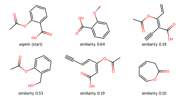
**Mutation** takes a molecule's SMILES, reorders it into one of its many equivalent non-canonical forms, converts it to SELFIES, replaces, inserts or deletes tokens at random, and decodes the result. Every SELFIES decodes, so each edit produces a valid molecule, and the reordering means the same starting structure produces edits at different positions in the graph. **Interpolation** aligns the SELFIES strings of two molecules and changes the differing positions, producing a **chemical path** between them from which a median molecule can be selected. Mutation is how the local chemical space for the MMACE counterfactuals of the [explainability](10_explainability.qmd) chapter is generated.
The cell below applies the mutation procedure to aspirin, and contrasts it with single-character edits made directly to the SMILES string.
```{python}
#| label: fig-stoned-mutation
#| fig-cap: "STONED mutation applied to aspirin. Each single-token edit of the SELFIES string decodes to a real molecule, with Tanimoto similarity to the starting structure shown below each. The counts printed above compare this with editing the SMILES string directly."
import numpy as np
import selfies as sf
from rdkit import Chem, RDLogger
from rdkit.Chem import Draw, rdFingerprintGenerator
from rdkit.DataStructs import TanimotoSimilarity

RDLogger.DisableLog("rdApp.*")
rng = np.random.default_rng(7)

start = "CC(=O)Oc1ccccc1C(=O)O"                       # aspirin
alphabet = sorted(sf.get_semantic_robust_alphabet())
fpgen = rdFingerprintGenerator.GetMorganGenerator(radius=2, fpSize=2048)


def similarity(a, b):
    fa, fb = (fpgen.GetFingerprint(Chem.MolFromSmiles(s)) for s in (a, b))
    return TanimotoSimilarity(fa, fb)


def stoned_mutate(smiles):
    """Reorder the SMILES, encode to SELFIES, replace one token, decode again."""
    mol = Chem.MolFromSmiles(smiles)
    order = rng.permutation(mol.GetNumAtoms()).tolist()
    reordered = Chem.MolToSmiles(Chem.RenumberAtoms(mol, order), canonical=False)
    tokens = list(sf.split_selfies(sf.encoder(reordered)))
    tokens[int(rng.integers(len(tokens)))] = alphabet[int(rng.integers(len(alphabet)))]
    return sf.decoder("".join(tokens))


def smiles_mutate(smiles):
    """Replace one character of the SMILES string with another legal SMILES character."""
    chars = list(smiles)
    chars[int(rng.integers(len(chars)))] = "CNOFcnos()[]=#123456"[int(rng.integers(20))]
    return "".join(chars)


def parses(smiles):
    mol = Chem.MolFromSmiles(smiles)
    return mol is not None and mol.GetNumAtoms() > 0


canonical = Chem.CanonSmiles(start)
mols, legends = [Chem.MolFromSmiles(start)], ["aspirin (start)"]
while len(mols) < 6:
    smi = stoned_mutate(start)
    if parses(smi) and Chem.CanonSmiles(smi) != canonical:
        mols.append(Chem.MolFromSmiles(smi))
        legends.append(f"similarity {similarity(start, smi):.2f}")

trials = 500
ok_selfies = sum(parses(stoned_mutate(start)) for _ in range(trials))
ok_smiles = sum(parses(smiles_mutate(start)) for _ in range(trials))
print(f"single-token SELFIES edits giving a molecule:    {ok_selfies}/{trials}")
print(f"single-character SMILES edits giving a molecule: {ok_smiles}/{trials}")

Draw.MolsToGridImage(mols, molsPerRow=3, subImgSize=(250, 200), legends=legends)
```
Every SELFIES edit produces a molecule, while the great majority of SMILES edits produce a string that no toolkit will parse. The Tanimoto similarities also show that a single token can change a great deal, since replacing one symbol may substitute an entire branch or ring closure rather than a single atom.
These two operations are used in the genetic algorithm JANUS [@nigam2022janus]: SELFIES mutation supplies the mutation step and SELFIES interpolation the crossover step.
The remainder of the chapter covers models which learn a distribution instead of searching over explicit molecular structures.
## Deep Generative Models
A deep generative model samples a vector $\mathbf{z}$ from a simple **noise** distribution, usually uniform or Gaussian, and transforms it into a realistic-looking sample $\tilde{x}$. The noise carries no information about molecules, which comes only from the model's network that has learned to map noise onto the region of chemical space that is covered by its training data.
Three symbols need to be kept apart: $x$ is an original data point, $\hat{x}$ a *reconstruction* of it as produced by the autoencoders of the [unsupervised learning](11_unsupervised_learning.qmd) chapter, and $\tilde{x}$ a *generated* sample corresponding to no particular input. Three relevant model families will be discussed here: variational autoencoders, diffusion models and generative language models.
### Variational autoencoders
Sampling a latent space is already possible with **principal component analysis** from the [unsupervised learning](11_unsupervised_learning.qmd) chapter. Each component comes with an explained variance, so its score can be treated as a Gaussian with that variance; drawing one sample per component and transforming back to feature space yields a data point that was never in the dataset. Applied to face images, this generates recognizable new faces.
An autoencoder replaces the fixed linear map with a learned non-linear one, but the analogy then stops working. It is trained only to reconstruct, and nothing constrains where the training points land in the latent space, so a randomly drawn point is likely to fall in a region the decoder was never trained on, where its output is not meaningful.
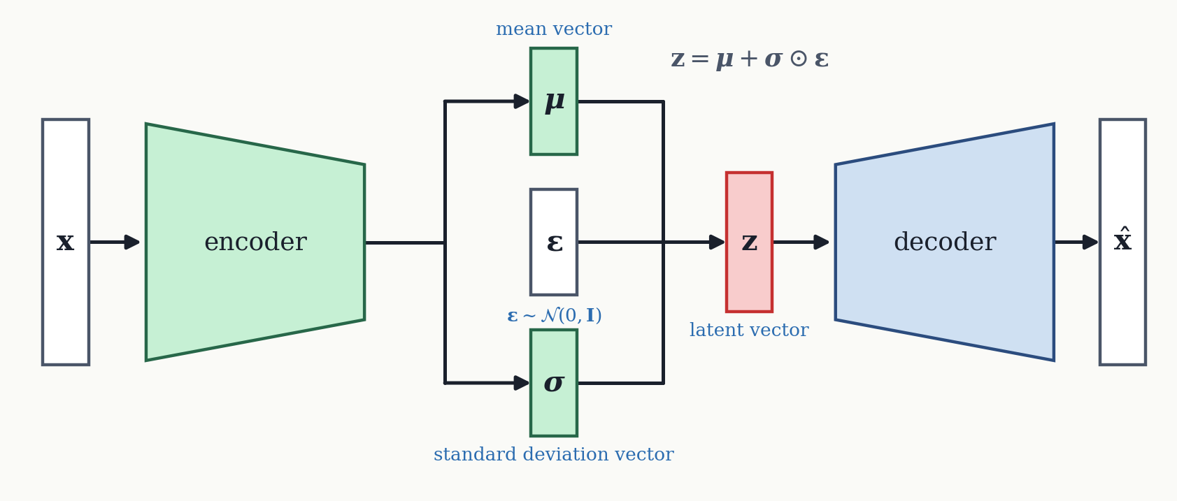
A **variational autoencoder** [@kingma2014vae] restores the property by making the encoding probabilistic. Instead of a single point, the encoder outputs two vectors, a **mean** $\boldsymbol{\mu}$ and a **standard deviation** $\boldsymbol{\sigma}$, together called the **codings**. The **latent vector** $\mathbf{z}$ passed to the decoder is drawn from the Gaussian $\mathcal{N}(\boldsymbol{\mu}, \boldsymbol{\sigma}^2)$ they define. Training proceeds one sample at a time: an example is encoded, a point $\mathbf{z}$ is sampled from the resulting distribution, the decoder reconstructs from it, and the weights are updated.
The loss has two terms that fulfill two different functions,
$$\mathcal{L} = -\frac{1}{2}\sum_{i}\left(1 + \log \sigma_i^2 - \sigma_i^2 - \mu_i^2\right) + \mathcal{L}_{\text{MSE}},$$
where the first is the **distribution loss** that punishes divergence from a standard Gaussian and the second the ordinary **reconstruction loss**. The reconstruction term alone would let the encoder scatter the codings anywhere; the distribution term forces the latent space into a Gaussian shape with no unused gaps, so new data can be generated by drawing $\mathbf{z}$ from that Gaussian and decoding it.
Sampling inside a network would ordinarily block backpropagation, since there is no gradient through a random draw. The **reparameterization trick** moves the randomness into an input instead, writing
$$\mathbf{z} = \boldsymbol{\mu} + \boldsymbol{\sigma}\odot\boldsymbol{\varepsilon}, \qquad \boldsymbol{\varepsilon}\sim\mathcal{N}(0, \mathbf{I}).$$
For a fixed draw of $\boldsymbol{\varepsilon}$ this is a differentiable expression in $\boldsymbol{\mu}$ and $\boldsymbol{\sigma}$, so gradients reach the encoder as usual, while drawing a fresh $\boldsymbol{\varepsilon}$ at every step keeps the procedure stochastic.
{#fig-vae width=95%}
This means both the encoder and decoder are deterministic networks, so the same input always gives the same $\boldsymbol{\mu}$ and $\boldsymbol{\sigma}$ and the same latent point always gives the same output. However, at the latent layer randomness enters the architecture with a different $\mathbf{z}$ sampled on every pass, so the same input can be reconstructed slightly differently each time. This yields a continuous latent space to be sampled from to generate data that is not in the training set but meaningful.
Applying this to molecules requires an encoder and decoder that can handle molecular representations, usually a sequence model over SMILES such as the recurrent networks of the [language models](09_language_models.qmd) chapter, although the original chemical variational autoencoder of @gomezbombarelli2018vae used a convolutional encoder with a recurrent decoder. Each molecule then has its own $\boldsymbol{\mu}$ and $\boldsymbol{\sigma}$, and the decoder turns any latent point back into a SMILES string.
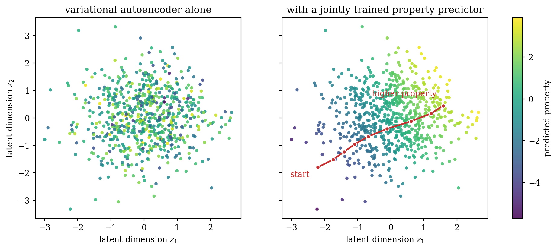
Trained on a drug-like dataset, the distribution loss alone gives a roughly Gaussian latent space that can be sampled, but the arrangement within it carries no useful information. Attaching a **property predictor**, a small feed-forward network trained jointly on the latent vectors, **orders** the space by the predicted property.
```{python}
#| label: fig-latent-space
#| fig-cap: "Illustration of a latent space coloured by a molecular property, using synthetic data. Trained on reconstruction and the distribution loss alone (left), the property is spread across the space with no spatial structure. Trained jointly with a property predictor (right), the space becomes ordered by the property, so gradient ascent in the latent space (red path) moves toward better molecules."
import numpy as np
import matplotlib.pyplot as plt

plt.rcParams.update({"font.family": "serif"})
rng = np.random.default_rng(3)

z = rng.normal(0, 1, size=(700, 2))
ordered = 1.5 * z[:, 0] + 0.8 * z[:, 1] + 0.3 * np.sin(2 * z[:, 0])
scrambled = rng.permutation(ordered)   # same property values, no spatial ordering

fig, axes = plt.subplots(1, 2, figsize=(11, 4.5), sharex=True, sharey=True)
for ax, values, title in ((axes[0], scrambled, "variational autoencoder alone"),
                          (axes[1], ordered, "with a jointly trained property predictor")):
    sc = ax.scatter(z[:, 0], z[:, 1], c=values, cmap="viridis", s=16,
                    alpha=0.85, edgecolors="none")
    ax.set_title(title, fontsize=12)
    ax.set_xlabel("latent dimension $z_1$")
axes[0].set_ylabel("latent dimension $z_2$")

# gradient ascent, which only makes sense on the ordered space
path = [np.array([-2.2, -1.8])]
for _ in range(8):
    p = path[-1]
    path.append(p + 0.35 * np.array([1.5 + 0.6 * np.cos(2 * p[0]), 0.8]))
path = np.array(path)
axes[1].plot(path[:, 0], path[:, 1], "-o", color="#c53030", lw=2, ms=5,
             markeredgecolor="white")
axes[1].annotate("start", path[0], textcoords="offset points", xytext=(-34, -12),
                 fontsize=10, color="#c53030")
axes[1].annotate("higher property", path[-1], textcoords="offset points", xytext=(-8, 12),
                 fontsize=10, color="#c53030", ha="right")

cb = fig.colorbar(sc, ax=axes.tolist(), fraction=0.035)
cb.set_label("predicted property")
plt.show()
```
That ordering turns molecular design into continuous optimization. Gradient ascent in the latent space moves toward higher predicted values, and the decoder converts the endpoint back into a molecule. Interpolating between two latent codes gives compounds with intermediate properties, a similar operation as STONED performs on strings but in a learned space.
A variational autoencoder compresses a molecule into a small latent vector and decodes it in a single step. The next family keeps the latent representation the same size as the data and builds the sample gradually instead.
### Diffusion models
A **diffusion model** is trained to remove noise. The procedure starts from a dataset in the domain of interest, molecules for instance, and perturbs those samples by adding Gaussian noise. The network is then trained on an ordinary supervised problem: given a noised sample as input, predict the noise that was added. The training set contains samples noised to **many different levels**, from barely perturbed to almost pure noise, so the network learns to denoise at every stage rather than at one. Once trained, it can be applied repeatedly to turn noise into data.
The equations below describe the standard formulation [@ho2020ddpm] and are given for orientation rather than memorization. Noise is added over a sequence of time steps, each perturbing the previous state by a small variance $\beta_t$ fixed by a schedule, and the steps compose into a closed form that jumps straight from the clean sample to any time $t$,
$$q(\mathbf{x}_t \mid \mathbf{x}_0) = \mathcal{N}\big(\sqrt{\bar{\alpha}_t}\,\mathbf{x}_0,\ (1 - \bar{\alpha}_t)\mathbf{I}\big), \qquad \alpha_t = 1-\beta_t, \quad \bar{\alpha}_t = \prod_{i=1}^{t}\alpha_i,$$
where $\bar{\alpha}_t$ tunes between the original sample at $\bar{\alpha}_0 = 1$ and pure noise at $\bar{\alpha}_T = 0$. The training set is built by drawing a noise level at random for each sample and applying it.
Generation reverses the process. A sample $\mathbf{x}_T$ is drawn from $\mathcal{N}(0, \mathbf{I})$ and the trained network $\boldsymbol{\varepsilon}_\theta$ is applied repeatedly, working backwards in time,
$$\mathbf{x}_{t-1} = \frac{1}{\sqrt{\alpha_t}}\left(\mathbf{x}_t - \frac{\beta_t}{\sqrt{1-\bar{\alpha}_t}}\,\boldsymbol{\varepsilon}_\theta(\mathbf{x}_t, t)\right) + \sqrt{\beta_t}\,\mathbf{z}.$$
At each step the network predicts the noise present and a portion of it is removed. The final term adds a little fresh Gaussian noise, which makes generation non-deterministic: running the same model twice gives two different results. The number of steps is often in the thousands.
The widget below applies the closed-form expression to paracetamol, drawn in two dimensions with explicit hydrogens. Each atom carries a position and an atom type, both noised on the same schedule, while the bonds are held fixed so the geometry distorts while connectivity persists. The time direction switches between adding noise and removing it.
```{shinylive-python}
#| standalone: true
#| viewerHeight: 660
from shiny import App, render, ui
import matplotlib
import matplotlib.pyplot as plt
import numpy as np
matplotlib.rcParams.update({
"font.family": "serif",
"figure.facecolor": "#fafaf7",
"axes.facecolor": "#fafaf7",
"axes.grid": True,
"grid.alpha": 0.3,
})
ELEMENTS = ["C", "N", "O", "H"]
ECOLOR = ["#4a5568", "#2b6cb0", "#c53030", "#e2e8f0"]
ETEXT = ["white", "white", "white", "#1a202c"]
ESIZE = [300, 300, 300, 165]
# Paracetamol, CC(=O)Nc1ccc(O)cc1, with explicit hydrogens. The 2D coordinates were
# generated once with RDKit and pasted here, since RDKit is not available in the browser.
X0 = np.array([
[-1.685, -0.006], [-1.060, 0.157], [-0.888, 0.781], [-0.606, -0.303],
[0.020, -0.139], [0.191, 0.484], [0.817, 0.647], [1.271, 0.187],
[1.896, 0.350], [1.099, -0.436], [0.474, -0.600], [-2.311, -0.169],
[-1.848, 0.620], [-1.522, -0.631], [-0.777, -0.926], [-0.263, 0.944],
[0.988, 1.270], [2.350, -0.110], [1.553, -0.896], [0.302, -1.223],
])
BONDS = [(0, 1), (1, 2), (1, 3), (3, 4), (4, 5), (5, 6), (6, 7), (7, 8), (7, 9),
(9, 10), (10, 4), (0, 11), (0, 12), (0, 13), (3, 14), (5, 15), (6, 16),
(8, 17), (9, 18), (10, 19)]
TYPES = np.array([0, 0, 2, 1, 0, 0, 0, 0, 2, 0, 0, 3, 3, 3, 3, 3, 3, 3, 3, 3])
H0 = np.eye(4)[TYPES] # atom types as one-hot vectors
T = 1000
betas = np.linspace(1e-4, 0.02, T)
alpha_bar = np.cumprod(1.0 - betas)
app_ui = ui.page_fluid(
ui.input_radio_buttons("direction", "Time direction",
{"fwd": "forward (add noise)", "rev": "reverse (remove noise)"},
selected="fwd", inline=True),
ui.input_slider("step", "Steps taken", min=0, max=T, value=0, step=10),
ui.input_slider("seed", "Noise sample", min=0, max=10, value=0, step=1),
ui.output_plot("diff_plot"),
)
def server(input, output, session):
@render.plot
def diff_plot():
step = int(input.step())
t = step if input.direction() == "fwd" else T - step
ab = 1.0 if t == 0 else float(alpha_bar[t - 1])
# epsilon depends only on the seed, so the reverse sweep retraces the
# forward one exactly and the molecule reappears.
rng = np.random.default_rng(int(input.seed()))
Xt = np.sqrt(ab) * X0 + np.sqrt(1 - ab) * rng.normal(0, 1, X0.shape)
Ht = np.sqrt(ab) * H0 + np.sqrt(1 - ab) * rng.normal(0, 1, H0.shape)
labels = Ht.argmax(axis=1)
fig, ax = plt.subplots(figsize=(7.2, 6.0))
ax.set_xlim(-3.6, 3.6)
ax.set_ylim(-3.2, 3.2)
ax.set_aspect("equal")
for i, j in BONDS:
ax.plot([Xt[i, 0], Xt[j, 0]], [Xt[i, 1], Xt[j, 1]],
"-", color="#a0aec0", lw=1.8, alpha=0.85, zorder=2)
for k in range(len(Xt)):
lab = labels[k]
ax.scatter(Xt[k, 0], Xt[k, 1], s=ESIZE[lab], color=ECOLOR[lab],
edgecolors="#4a5568" if lab == 3 else "white",
linewidths=0.8, zorder=4)
ax.text(Xt[k, 0], Xt[k, 1], ELEMENTS[lab], color=ETEXT[lab],
ha="center", va="center",
fontsize=9 if lab == 3 else 11, fontweight="bold", zorder=5)
ax.set_title(f"t = {t} of {T} " + r"$\bar{\alpha}_t$ = " + f"{ab:.3f}",
fontsize=13, fontweight="bold")
fig.tight_layout()
return fig
app = App(app_ui, server)
```
Running forward, $\bar{\alpha}_t$ falls to zero and the molecule dissolves: the atoms scatter and the element labels scramble as the noised type vectors lose their original largest component. Running in reverse, both recover. The reverse sweep here replays exactly the noise that was added, which is why it reconstructs the molecule perfectly. A trained model has no such record and must *predict* the noise at every step from the noisy sample alone.
A molecule is defined by where its atoms are **and** what they are, so positions and atom types are noised and denoised together, and a sample is only usable if both come out consistent. More sophisticated models also account for the fact that a rotated or translated molecule is the same molecule, building the equivariance discussed in the [graph models](08_graph_models.qmd) chapter into the denoising network [@hoogeboom2022equivariant].
The most prominent application is **AlphaFold 3** [@abramson2024alphafold3], which predicts three-dimensional structures for biomolecular complexes: proteins together with nucleic acids, ligands and ions, rather than a protein sequence alone. Most of the architecture turns those inputs into a rich representation and lies beyond this chapter, but the structure itself comes from a diffusion module that starts from noise and runs roughly 200 denoising steps.
Because generation is stochastic, one input does not give one output: the model produces several predictions per random seed and a separate **confidence module** ranks them. Confidence is also reported for each part of the structure, and the least certain regions are typically the flexible or disordered parts of the protein, which have no single well-defined structure to predict.
### Generative language models
A molecule written as SMILES is a sequence, and the [language models](09_language_models.qmd) chapter covered how sequences are generated: **autoregressively**, one token at a time, starting from a begin of sequence token and stopping when the model emits a special end token. Each token's probability is conditioned on all tokens generated so far, and tokens are **sampled** from that distribution rather than always taken at the maximum, which is what makes the output varied. Applying this to SMILES to build focused molecule libraries goes back to @segler2018generating.
Sampling from such a model gives molecules resembling its training set, which is unconditional generation. Steering it toward desired properties is what **REINVENT** [@olivecrona2017reinvent] adds, using reinforcement learning. A **prior** network is first trained on a large set of SMILES, typically from ChEMBL, so that it generates plausible drug-like molecules. It is then **copied** to an **agent** network, and only the agent is ever updated: the agent generates molecules, a scoring function evaluates them, and the weights are adjusted so that high-scoring molecules become more likely. The loss for a generated sequence $T$ is
$$\mathcal{L}(T) = \big(\log P_{\text{aug}}(T) - \log P_{\text{agent}}(T)\big)^2, \qquad \log P_{\text{aug}}(T) = \log P_{\text{prior}}(T) + \sigma\, S(T),$$
where $S$ is the scoring function and $\sigma$ sets how strongly the score pulls. The **prior stays frozen** throughout, and that is the point of the design. Without it the agent would drift toward whatever region of string space maximizes the score, which is unlikely to contain reasonable molecules at all. The prior anchors the agent to the distribution it started from while the score moves it within that distribution.
@li2023organic use this to search for singlet fission materials for more efficient solar cells. Their scoring function combines cheminformatics criteria, namely molecular weight, rotatable bond count, substructure matches and a synthesizability score, with an electronic scoring function from quantum chemistry. Reporting the outcome as a Pareto front of total score against synthesizability, rather than as a single best molecule, makes the trade-off explicit. REINVENT 4 [@loeffler2024reinvent], the current version, packages the same machinery for the design tasks introduced at the start of this chapter.
Both the frozen prior and the Pareto front are guards against the same underlying failure, which affects every model in this chapter and is worth treating on its own.
## Reward Hacking
A generative model optimizes the score it is given, not the goal the chemist has in mind. Where the two come apart, a capable generator will find the gap and exploit it. This failure is called **reward hacking**, and it arises in two ways.
The score may be wrong. Scoring functions are frequently predictive models themselves, and a generative search pushes deliberately into regions of chemical space far from their training data, which is exactly where their predictions are least reliable. The [applicability domain](04_model_evaluation.qmd) of the scoring model therefore bounds the search built on top of it.
Or the score may be incomplete. Whatever a scoring function leaves out because maybe it is expensive to calculate or impossible to formalize is left unconstrained, and an optimizer might trade away real world applicability for modest gains in score. A score built only from predicted binding affinities can return molecules that no synthetic route can reach, that decompose on the bench, or that bind as readily to everything else as to the intended target.
A better generator fixes neither problem. Building validity and synthesizability into the score, reporting a Pareto front rather than a single number, and anchoring the search to a prior distribution all help, but the scoring function sets the ceiling.
## Summary
- **Predictive vs. generative models.** A predictive model learns $p(y \mid x)$ to score a molecule; a generative model learns $p(x)$ so new molecules can be sampled from it, needing only examples and no labels. Generation may be conditioned on a scaffold, fragment, prompt or property target, and inverse design refers to starting from the desired properties instead of screening for them.
- **Genetic algorithms** evolve a population through fitness evaluation, selection, crossover and mutation. They need no training data of their own and remain a strong baseline. Their behaviour balances exploration against exploitation, set by the population size, the mutation rate and size, and the amount of crossover.
- **SELFIES and STONED.** Every SELFIES string decodes to a valid molecule, which lets STONED mutate a molecule by editing tokens and interpolate between two along a chemical path. These are operations rather than a search algorithm; JANUS is the genetic algorithm built on them.
- **Variational autoencoders** encode an input to a mean vector and a standard deviation vector and sample the latent vector from the Gaussian these define. A reconstruction loss and a distribution loss together give a latent space smooth enough to sample and interpolate in, and a jointly trained property predictor orders it so it can be optimized over.
- **Diffusion models** are trained to predict the noise added to a sample, using data noised to many different levels, and generate by denoising iteratively from pure noise. For molecules, coordinates and atom types are denoised together. AlphaFold 3 predicts biomolecular complexes this way.
- **Generative language models** produce SMILES autoregressively. REINVENT steers such a model by reinforcement learning, copying a frozen prior into a trainable agent so the score improves without the agent leaving the chemical space the prior describes.
- **The scoring function sets the ceiling.** Generated molecules are only as good as the function used to rank them, and a capable generator can exploit a mismatch between a high score and low real-world suitability of a molecule. This is reward hacking and can arise from erroneous model predictions used in the scoring or dimensions missing from the score altogether. Building synthesizability and other realistic constraints into the score, and reporting trade-offs as a Pareto front rather than a single number, is what keeps the output useful.