---
title: "Interpretability and Explainability"
format:
html:
code-fold: true
toc: true
theme: cosmo
jupyter: python3
---
A trained model gives predictions, but **explainable AI** (XAI) analyses *why*. Understanding how a model constructs its predictions lets us trust it and troubleshoot it. If a model has learned accurate predictions, it might be possible to extract chemical insight. Yet, explanations have to be treated with caution as they are fully based on correlations and not on causal effects.
## Defining an explanation
An explanation is an answer to a why-question. Good explanations should fulfill the following properties:
- **Contrastive** — they compare against a reference
- **Selective** — they cite just a few, selected factors
- **Understandable** — they use the receiver's language
- **Truthful** — they match reality
The example explanation "Hexanol is more soluble in polar solvents than hexane *because it has an alcohol group*" works because it is contrastive and selective.
Explainations can be important for multiple reasons.
First of all, they can help to **build trust** among end users who are frequently unfamiliar with the details of the modeling algorithms. Model predictions together with chemical explanations can provide an intuitive perspective to a chemist on how the model constructed its prediction.
Another benefit of explanations is that they can **expose failure modes** of a model. Analyzing model explanations for well understood chemical problems may highlight weaknesses in the model's learning or even expose unintended exploitation of irrelevant attributes.
Lastly, explanations are **necessary in regulatory settings**, e.g. toxicity assessments where a model must justify its predictions.
## Explainability methods
Two axes organize the field:
- **Model-specific vs. model-agnostic.** Model-specific methods exploit a particular model's internal variables while model-agnostic methods treat the model as a black box and can be applied universally.
- **Global vs. local.** Global methods explain the model's *overall* behavior across the dataset; local methods explain a *single* prediction.
Models sit on an interpretability spectrum [@Esterhuizen_2022]:
- **Black box** — internals opaque
- **Grey box** — opaque, but with a well-established way of extracting information
- **Glass box** — directly inspectable
The choice of an ML model is constrained by a flexibility–interpretability trade-off: The more flexible the model, the less interpretable it tends to be.
Highly flexible models such as deep learning, SVMs or boosting algorithms are very difficult to interpret.
In contrast, very interpretable models such as (regularized) linear regression or decision trees offer only low modeling flexibility.
Bagging algorithms (random forests) provide a compromise between flexibility and interpretability, as a grey box model.
## Explaining linear models
Coefficients from linear models are interpretable **with cautions**:
- Features must be on the **same scale** for coefficients to be comparable
- Simple explanations require **sparse** models (Lasso, feature selection)
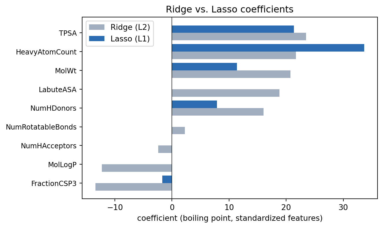
A linear model's coefficients correspond to its explanation. The example below predicts the boiling temperature of 72 common organic molecules (with experimental values sourced from PubChem) from RDKit descriptors, scaled so the coefficients are comparable. We fit two regularized models: **Ridge**, which shrinks all coefficients toward zero but keeps every descriptor, and **Lasso**, which drives weak coefficients *exactly* to zero. As anticipated, Lasso keeps only a small number of features with non-zero coefficients, while Ridge keeps non-zero coefficients for all features.
```{python}
#| label: feature-importance
#| fig-cap: "Ridge vs. Lasso coefficients for a boiling-point model built from molecular descriptors. Both penalize large coefficients; Lasso (L1) additionally zeros out the redundant ones for a sparse, readable model."
import numpy as np
import pandas as pd
import matplotlib.pyplot as plt
from rdkit import Chem
from rdkit.Chem import Descriptors, Crippen
from sklearn.preprocessing import StandardScaler
from sklearn.linear_model import Ridge, Lasso

# Boiling points (deg C) and SMILES sourced from PubChem; see figures/boiling_points.csv
data = pd.read_csv("figures/boiling_points.csv")

descriptors = {"MolWt": Descriptors.MolWt, "MolLogP": Crippen.MolLogP,
               "TPSA": Descriptors.TPSA, "NumHDonors": Descriptors.NumHDonors,
               "NumHAcceptors": Descriptors.NumHAcceptors,
               "NumRotatableBonds": Descriptors.NumRotatableBonds,
               "HeavyAtomCount": Descriptors.HeavyAtomCount,
               "LabuteASA": Descriptors.LabuteASA,
               "FractionCSP3": Descriptors.FractionCSP3}
names = np.array(list(descriptors))

X_raw = np.array([[f(Chem.MolFromSmiles(smi)) for f in descriptors.values()]
                  for smi in data.smiles])
y = data.bp_celsius.values
X = StandardScaler().fit_transform(X_raw)

ridge = Ridge(alpha=10.0).fit(X, y)
lasso = Lasso(alpha=12.0).fit(X, y)

order = np.argsort(ridge.coef_)
y_pos = np.arange(len(names))
fig, ax = plt.subplots(figsize=(7, 4.2))
ax.barh(y_pos - 0.2, ridge.coef_[order], height=0.4, color="#a0aec0", label="Ridge (L2)")
ax.barh(y_pos + 0.2, lasso.coef_[order], height=0.4, color="#2b6cb0", label="Lasso (L1)")
ax.axvline(0, color="black", lw=0.6)
ax.set_yticks(y_pos); ax.set_yticklabels(names[order], fontsize=9)
ax.set_xlabel("coefficient (boiling point, standardized features)")
ax.set_title("Ridge vs. Lasso coefficients")
ax.legend()
fig.tight_layout()
plt.show()
```
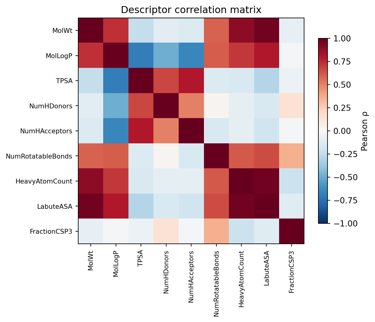
Importances and coefficients can mislead when features are **correlated**, because the model can split credit arbitrarily among them. A pairwise **correlation matrix** or **variance inflation factors** help diagnose collinearity.
The heatmap below shows the molecular descriptors are far from independent: molecular weight (MolWt), heavy-atom count and Labute surface area (LabuteASA) all measure *size* and are correlated above 0.9. That is exactly why Lasso dropped `LabuteASA`: with `MolWt` already in the model it carries almost no new information.
```{python}
#| label: collinearity
#| fig-cap: "Correlation matrix of the molecular descriptors — size-related descriptors are correlated above 0.9, warning against over-reading any single coefficient."
import matplotlib.pyplot as plt

corr = np.corrcoef(X_raw, rowvar=False)

fig, ax = plt.subplots(figsize=(6.5, 5.5))
im = ax.imshow(corr, cmap="RdBu_r", vmin=-1, vmax=1)
ax.set_xticks(range(len(names))); ax.set_yticks(range(len(names)))
ax.set_xticklabels(names, rotation=90, fontsize=8)
ax.set_yticklabels(names, fontsize=8)
fig.colorbar(im, ax=ax, label="Pearson \u03c1", shrink=0.8)
ax.set_title("Descriptor correlation matrix")
fig.tight_layout()
plt.show()
```
The general recommendations:
- be careful interpreting importances
- scale and standardize features
- account for collinearity
- check **stability** by re-estimating importances on resampled data.
## Explaining black box models
### SHAP analysis
**SHapley Additive exPlanations** is the most-used model-agnostic, local method. Borrowing from game theory, it treats the features as players in a game and fairly assigns each one "credit" for the prediction. The explanation for one sample, $g(\mathbf{x}')$, is a linear sum of per-feature attributions:
$$
g(\mathbf{x}') = \phi_0 + \sum_{j=1}^{M} \phi_j ,
$$
where $\phi_0$ is the **mean prediction** over the dataset and each $\phi_j$ is feature $j$'s contribution that pushes this particular prediction above or below the average.
Global explanations are obtained by aggregating all local explanations to create summary metrics describing the full dataset.
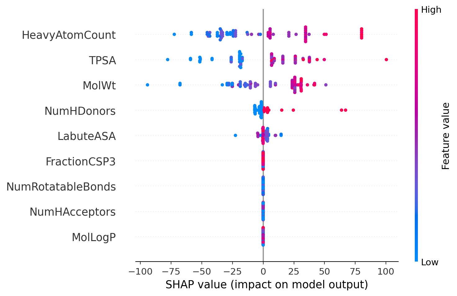
To see this on real data we train a **simple decision tree** to predict the boiling points of the 72 molecules above, then call `shap.TreeExplainer` to get an exact attribution $\phi_j$ for every descriptor of every molecule.
The **summary (beeswarm) plot** shows the full *distribution* of local SHAP values for each feature — one dot per molecule, placed by its SHAP value (its °C contribution to that molecule's predicted boiling point) and colored by the feature's value (low → blue, high → red):
```{python}
#| label: shap-summary
#| fig-cap: "SHAP summary (beeswarm) plot: the distribution of local SHAP values per descriptor. Each dot is one molecule, colored by the descriptor's value."
import shap
from sklearn.tree import DecisionTreeRegressor

tree = DecisionTreeRegressor(max_depth=4, random_state=0).fit(X_raw, y)
explainer = shap.TreeExplainer(tree)
shap_values = explainer.shap_values(X_raw)

shap.summary_plot(shap_values, X_raw, feature_names=names, show=False)
plt.tight_layout()
plt.show()
```
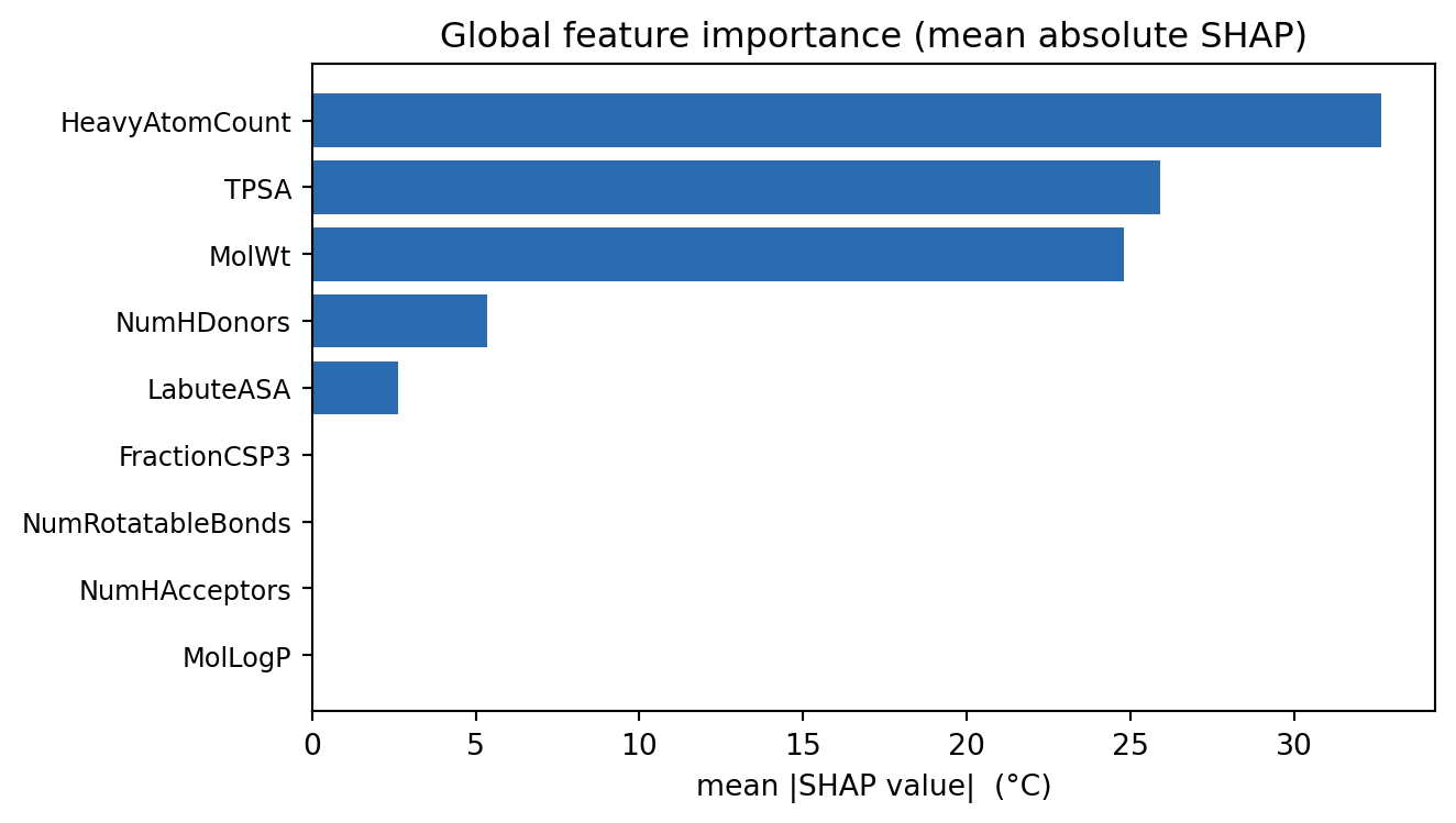
Each red `MolWt`/`TPSA` dot sitting to the right confirms the chemistry: heavier, more polar molecules boil higher. Collapsing every feature's distribution to its **mean absolute SHAP value** turns these local explanations into a single **global importance** that ranks the descriptors across the whole dataset:
```{python}
#| label: shap-global
#| fig-cap: "Global SHAP analysis: the mean absolute SHAP value per descriptor (in °C), aggregating all 72 local explanations."
global_imp = np.abs(shap_values).mean(axis=0)   # mean |SHAP| per feature, in C
gorder = np.argsort(global_imp)
fig, ax = plt.subplots(figsize=(7, 4.0))
ax.barh(np.arange(len(names)), global_imp[gorder], color="#2b6cb0")
ax.set_yticks(np.arange(len(names))); ax.set_yticklabels(names[gorder], fontsize=9)
ax.set_xlabel("mean |SHAP value|  (°C)")
ax.set_title("Global feature importance (mean absolute SHAP)")
fig.tight_layout()
plt.show()
```
### Deep learning with gradients
For neural networks a local explanation can be obtained by analyzing the **gradient of the output with respect to the input**. These gradients describe how much nudging each input feature changes the prediction.
This approach is applicable also to specialized deep learning methods such as image models (importance per pixel) or predictions on molecules (importance per atom and bond).
### Counterfactuals
Counterfactual-based interpretability takes a complementary approach and asks: **what is the smallest change to the input that flips the prediction?**
For molecules, this means the smallest structural edit that changes the predicted class (or alters the regression output by $\Delta$). The distance is commonly measured by the Tanimoto distance in fingerprint space:
- **Classification:** minimize $d(x, x')$ such that $\hat{f}(x) \neq \hat{f}(x')$.
- **Regression:** minimize $d(x, x')$ such that $|\hat{f}(x) - \hat{f}(x')| \geq \Delta$.
A concrete realization is **MMACE** (Model-Agnostic Counterfactual Explanations), implemented in the [`exmol`](https://github.com/ur-whitelab/exmol) package [@Wellawatte_2022]. It expands chemical space around a base molecule, then returns the most *similar* molecule with the *opposite* prediction.
## Summary
Explainable AI asks *why* a model predicted what it did. The chapter covered:
- **What counts as an explanation.** A good explanation is contrastive and selective. Explanations build trust with non-expert users, expose failure modes on problems where the chemistry is already understood, and are required outright in regulatory settings.
- **Two axes of methods.** *Model-specific* methods exploit a model's internals, *model-agnostic* ones treat it as a black box; *global* methods describe overall behavior across the dataset, *local* ones a single prediction.
- **Flexibility costs interpretability.** Models sit on a spectrum from **glass box** (directly inspectable) through **grey box** (opaque, but with an established way to extract information) to **black box** (internals opaque) which runs opposite to model capability.
- **Linear models** explain themselves through their coefficients but only if the features are on the same scale and the model is sparse. Correlated features let the model split credit arbitrarily, so check collinearity and the stability of importances under resampling.
- **SHAP** treats features as players sharing credit for a prediction, giving exact local attributions that aggregate into global importances.
- **Gradients and counterfactuals** cover the rest: gradients report how much nudging each input moves a model's output, while counterfactuals ask for the smallest structural edit that flips the prediction.