---
title: "Molecular Representations"
format:
html:
code-fold: true
toc: true
theme: cosmo
jupyter: python3
filters:
- shinylive
---
The first step in any machine learning workflow for chemistry is converting molecules into numbers that a computer is able to *understand*. There is a hierarchy of representations with different trade-offs and containing different levels of information on the chemistry that is represented. One such scale that is broadly considered is the dimensionality of the representation:
- **1D** — the molecular composition
- **2D** — the molecular graph (topology)
- **2.5D** — the molecular graph with information on stereochemistry
- **3D** — the molecular geometry
- **4D** — the ensemble of molecular geometries
## Molecular Composition (1D)
The simplest representation is the **composition**: how many atoms of each element the molecule contains, with no connectivity (*e.g.*, C₉H₈O₄). It is mainly useful when no better representation is available, for instance when the structure of a sample is unknown. Its key limitation is that all isomers of a formula collapse onto a single representation.
## Molecules as Graphs (2D)
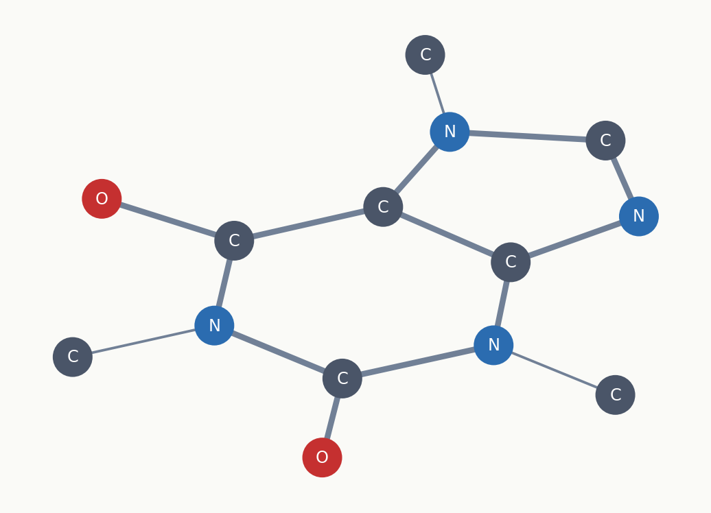
One chemically intuitive way to represent molecules is as graphs, where the electrons are assigned to the atoms and covalent bonds share their electrons between two atoms. This lets us treat molecules with concepts from mathematical graph theory, which models pairwise relations between objects. A graph in this context is made up of nodes (the atoms of a molecule) and edges (the bonds) that connect them. Based on this concept we can come up with various ways by which to encode the information of a graph in a machine-readable format such as adjacency matrices or line notations which will be the focus of the next section.
```{python}
#| label: fig-molecule-as-graph
#| fig-cap: "Caffeine drawn as a graph: atoms are nodes (coloured by element) and bonds are edges (thicker for double bonds). Hydrogens are implicit."
import matplotlib.pyplot as plt
import networkx as nx
from rdkit import Chem

plt.rcParams.update({"figure.facecolor": "#fafaf7", "axes.facecolor": "#fafaf7"})

mol = Chem.MolFromSmiles("Cn1cnc2c1c(=O)n(C)c(=O)n2C")   # caffeine

G = nx.Graph()
for atom in mol.GetAtoms():
    G.add_node(atom.GetIdx(), element=atom.GetSymbol())
for bond in mol.GetBonds():
    G.add_edge(bond.GetBeginAtomIdx(), bond.GetEndAtomIdx(),
               order=bond.GetBondTypeAsDouble())

colors = {"C": "#4a5568", "N": "#2b6cb0", "O": "#c53030"}
fig, ax = plt.subplots(figsize=(5.5, 4))
pos = nx.kamada_kawai_layout(G)
nx.draw_networkx_edges(G, pos, ax=ax, edge_color="#718096",
                       width=[1.4 if G.edges[e]["order"] == 1 else 3.2 for e in G.edges])
nx.draw_networkx_nodes(G, pos, ax=ax, node_size=430,
                       node_color=[colors[G.nodes[n]["element"]] for n in G.nodes])
nx.draw_networkx_labels(G, pos, ax=ax, font_size=9, font_color="white",
                        labels={n: G.nodes[n]["element"] for n in G.nodes})
ax.axis("off")
plt.tight_layout()
plt.show()
```
## SMILES
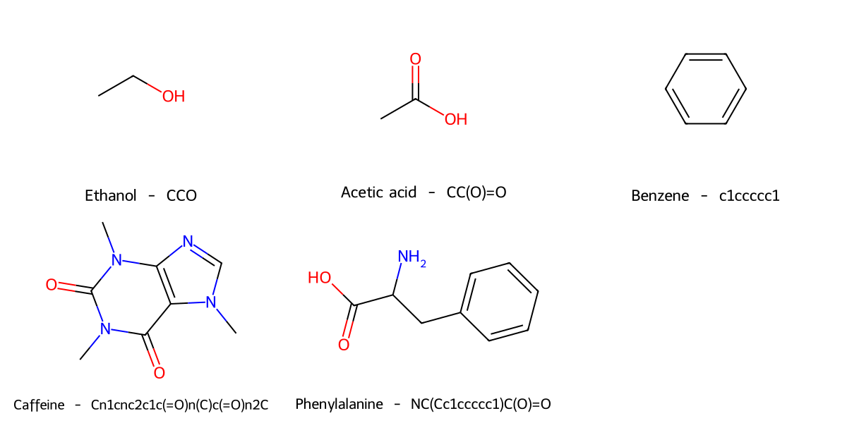
SMILES (Simplified Molecular Input Line Entry Specification) encodes a molecular graph as a linear string of characters. It is the most widely used line notation in cheminformatics.
The encoding follows a few rules: atoms are represented by their symbol, bonds by special characters (`=` for double, `#` for triple, omitted for single), branches in parentheses `()`, and ring closures with matching digits. Aromatic atoms use lowercase letters.
```{python}
#| label: smiles-demo
#| fig-cap: "Molecules generated from SMILES strings, rendered with RDKit."
from rdkit import Chem
from rdkit.Chem import Draw

smiles_examples = {
    "Ethanol": "CCO",
    "Acetic acid": "CC(O)=O",
    "Benzene": "c1ccccc1",
    "Caffeine": "Cn1cnc2c1c(=O)n(C)c(=O)n2C",
    "Phenylalanine": "NC(Cc1ccccc1)C(O)=O",
}

mols = [Chem.MolFromSmiles(s) for s in smiles_examples.values()]

# Keep each legend on one line: RDKit sizes the legend font to fit the tile
# width, so a two-line "name\nSMILES" legend collides with itself whenever the
# text is short enough to stay at full size.
legends = [f"{name}  -  {smi}" for name, smi in smiles_examples.items()]

opts = Draw.rdMolDraw2D.MolDrawOptions()
opts.legendFontSize = 22
opts.legendFraction = 0.18  # default 0.1 leaves the legend cramped
Draw.MolsToGridImage(mols, molsPerRow=3, subImgSize=(400, 300),
                     legends=legends, drawOptions=opts)
```
Note:
- SMILES strings are **not unique**: the same molecule can have many valid SMILES (e.g., `BrC(C)C` and `CC(C)Br` are both valid for 2-bromopropane). Canonicalization algorithms produce a single canonical SMILES per molecule, but these differ between toolkits.
- **Not all strings are valid**: random character sequences rarely correspond to real molecules.
- **Tautomers** have different SMILES: this can cause problems when comparing molecules.
## Fingerprints
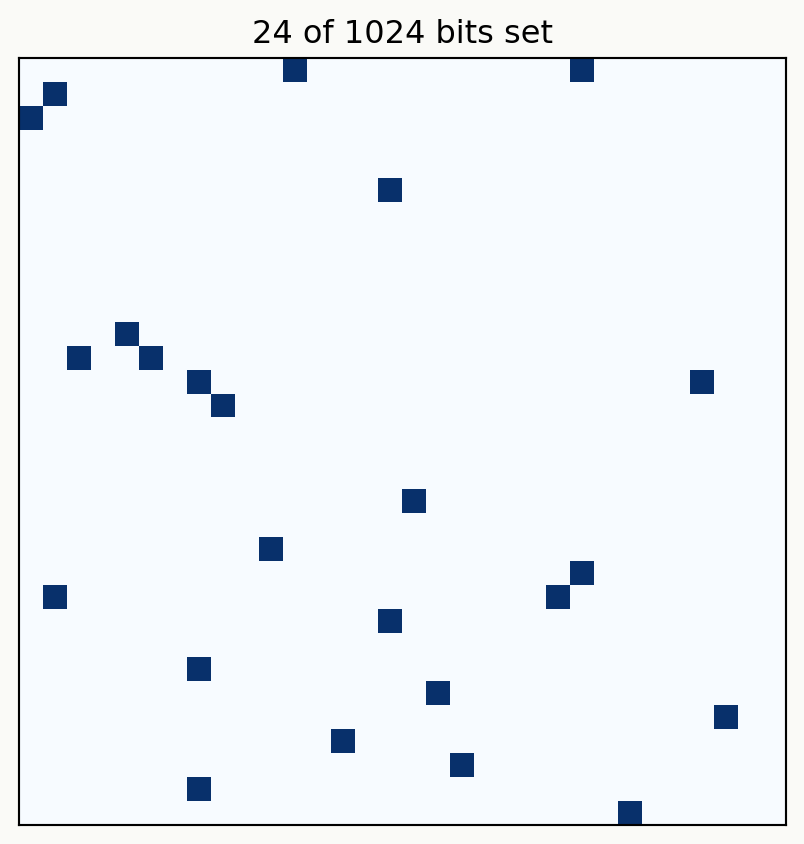
Fingerprints encode structural features of a molecule as a fixed-length vector of bits or counts. The most widely used is the **Morgan fingerprint**, closely related to the **ECFP** (Extended-Connectivity Fingerprint): both use the same Morgan algorithm below, but ECFP is one specific published parametrisation of it.
```{python}
#| label: fig-fingerprint-vector
#| fig-cap: "A Morgan fingerprint of aspirin (radius 2, 1024 bits), shown as the vector it is, folded to 32x32. Dark cells are set bits; only a few dozen of the 1024 positions are on."
import numpy as np
import matplotlib.pyplot as plt
from rdkit import Chem
from rdkit.Chem import AllChem

mol = Chem.MolFromSmiles("CC(=O)Oc1ccccc1C(=O)O")           # aspirin
bits = np.array(AllChem.GetMorganFingerprintAsBitVect(mol, radius=2, nBits=1024), dtype=int)

fig, ax = plt.subplots(figsize=(4.5, 4.5))
ax.imshow(bits.reshape(32, 32), cmap="Blues", vmin=0, vmax=1, interpolation="nearest")
ax.set_title(f"{bits.sum()} of 1024 bits set")
ax.set_xticks([]); ax.set_yticks([])
plt.tight_layout()
plt.show()
```
The algorithm works as follows:
1. Assign an initial identifier to each atom based on its properties (atomic number, degree, charge, etc.).
2. Iteratively update each atom's identifier by incorporating the identifiers of its neighbors, up to a specified **radius**.
3. Hash all collected identifiers into a bit vector of fixed **length**.
The two key parameters are:
- **Radius**: how many bonds away from each atom to consider. Radius 2 (ECFP4) and radius 3 (ECFP6) are most common. A larger radius captures more context, but the features become so specific that a bit may be set for only one molecule in the dataset, giving nothing to compare or generalize from.
- **Number of bits** (nBits): the length of the fingerprint vector. Common choices are 1024 or 2048. Shorter vectors are cheaper to store and faster to compare or train on, but cause more **bit collisions** (different substructures mapped to the same bit), losing information.
```{python}
#| label: morgan-demo
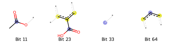
#| fig-cap: "Visualizing Morgan fingerprint bits for aspirin. Each highlighted region shows the atoms contributing to a particular bit."
from rdkit import Chem
from rdkit.Chem import Draw, AllChem

mol = Chem.MolFromSmiles("CC(=O)Oc1ccccc1C(=O)O")  # Aspirin
bi = {}
fp = AllChem.GetMorganFingerprintAsBitVect(mol, radius=2, nBits=1024, bitInfo=bi)

# Pick a few set bits to visualize
set_bits = list(bi.keys())[:4]

tpls = [(mol, bit, bi) for bit in set_bits]
Draw.DrawMorganBits(tpls, molsPerRow=4, legends=[f"Bit {b}" for b in set_bits])
```
## Tanimoto Similarity
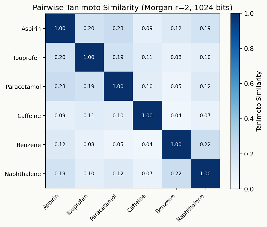
The **Tanimoto coefficient** is the standard way to measure similarity between two molecular fingerprints:
$$T_{AB} = \frac{c}{a + b - c}$$
where $a$ is the number of bits set in molecule A, $b$ is the number of bits set in molecule B, and $c$ is the number of bits set in both. The Tanimoto similarity ranges from 0 (no shared bits) to 1 (identical fingerprints). The corresponding distance is $D = 1 - T$.
For bit vectors this is identical to the **Jaccard index**, and the two names are used interchangeably. The equivalence holds only for bit vectors: Tanimoto also has a form for count fingerprints, where it is no longer the same quantity as Jaccard.
The **similar property principle** states that structurally similar molecules tend to have similar properties. This motivates virtual screening, clustering, and many other cheminformatics applications.
```{python}
#| label: tanimoto-demo
#| fig-cap: "Tanimoto similarity matrix for a set of molecules. Darker blue = more similar."
from rdkit import Chem, DataStructs
from rdkit.Chem import AllChem, Draw
import matplotlib.pyplot as plt
import numpy as np

smiles_list = [
    ("Aspirin", "CC(=O)Oc1ccccc1C(=O)O"),
    ("Ibuprofen", "CC(C)Cc1ccc(cc1)C(C)C(=O)O"),
    ("Paracetamol", "CC(=O)Nc1ccc(O)cc1"),
    ("Caffeine", "Cn1cnc2c1c(=O)n(C)c(=O)n2C"),
    ("Benzene", "c1ccccc1"),
    ("Naphthalene", "c1ccc2ccccc2c1"),
]

mols = [Chem.MolFromSmiles(s) for _, s in smiles_list]
fps = [AllChem.GetMorganFingerprintAsBitVect(m, 2, nBits=1024) for m in mols]
names = [n for n, _ in smiles_list]

n = len(fps)
sim_matrix = np.zeros((n, n))
for i in range(n):
    for j in range(n):
        sim_matrix[i, j] = DataStructs.TanimotoSimilarity(fps[i], fps[j])

fig, ax = plt.subplots(figsize=(6, 5))
im = ax.imshow(sim_matrix, cmap="Blues", vmin=0, vmax=1)
ax.set_xticks(range(n))
ax.set_xticklabels(names, rotation=45, ha="right", fontsize=9)
ax.set_yticks(range(n))
ax.set_yticklabels(names, fontsize=9)

for i in range(n):
    for j in range(n):
        ax.text(j, i, f"{sim_matrix[i,j]:.2f}", ha="center", va="center",
                fontsize=8, color="white" if sim_matrix[i,j] > 0.5 else "black")

plt.colorbar(im, label="Tanimoto Similarity")
plt.title("Pairwise Tanimoto Similarity (Morgan r=2, 1024 bits)")
plt.tight_layout()
plt.show()
```
Two things to read off the matrix. The values are low in absolute terms — even aspirin and paracetamol score well under 0.5 — so Tanimoto is not a percentage of shared structure and should be used to rank pairs rather than as an absolute score. And it measures shared substructure, not shared properties: aspirin and ibuprofen are both NSAIDs yet score low, which is exactly where the similar property principle fails.
### Interactive example: Tanimoto similarity
This widget demonstrates the Tanimoto calculation on two short bit vectors. Toggle bits on and off to see how the similarity changes.
```{shinylive-python}
#| standalone: true
#| viewerHeight: 620
from shiny import App, render, ui, reactive
import matplotlib.pyplot as plt
import matplotlib
import matplotlib.patches as mpatches
import numpy as np
matplotlib.rcParams.update({
"font.family": "serif",
"figure.facecolor": "#fafaf7",
"axes.facecolor": "#fafaf7",
"axes.grid": True,
"grid.alpha": 0.3,
})
all_bits = ["1", "2", "3", "4", "5", "6", "7", "8"]
app_ui = ui.page_fluid(
ui.input_checkbox_group("bitsA", "Molecule A bits", choices=all_bits,
selected=["1", "2", "3", "5"], inline=True),
ui.input_checkbox_group("bitsB", "Molecule B bits", choices=all_bits,
selected=["2", "3", "6", "7"], inline=True),
ui.output_plot("tanimoto_plot"),
)
def server(input, output, session):
@output
@render.plot
def tanimoto_plot():
set_a = set(input.bitsA())
set_b = set(input.bitsB())
a = len(set_a)
b = len(set_b)
c = len(set_a & set_b)
tanimoto = c / (a + b - c) if (a + b - c) > 0 else 0.0
fig, ax = plt.subplots(figsize=(8, 4))
ax.set_xlim(-0.5, 9.5)
ax.set_ylim(-0.5, 5.5)
ax.set_aspect("equal")
ax.axis("off")
cell_w = 0.85
cell_h = 0.8
gap = 0.1
start_x = 1.0
ax.text(0.3, 4.0, "A:", fontsize=14, fontweight="bold", color="#333333", va="center")
ax.text(0.3, 2.8, "B:", fontsize=14, fontweight="bold", color="#333333", va="center")
for i, bit in enumerate(all_bits):
x = start_x + i * (cell_w + gap)
in_a = bit in set_a
in_b = bit in set_b
both = in_a and in_b
# Row A
color_a = "#276749" if both else ("#2b6cb0" if in_a else "#eeeeee")
text_color_a = "white" if in_a else "#aaaaaa"
rect_a = mpatches.FancyBboxPatch((x, 3.65), cell_w, cell_h, boxstyle="round,pad=0.05",
facecolor=color_a, edgecolor="#cccccc", linewidth=1)
ax.add_patch(rect_a)
ax.text(x + cell_w / 2, 4.05, "1" if in_a else "0",
ha="center", va="center", fontsize=12, color=text_color_a)
# Row B
color_b = "#276749" if both else ("#c53030" if in_b else "#eeeeee")
text_color_b = "white" if in_b else "#aaaaaa"
rect_b = mpatches.FancyBboxPatch((x, 2.45), cell_w, cell_h, boxstyle="round,pad=0.05",
facecolor=color_b, edgecolor="#cccccc", linewidth=1)
ax.add_patch(rect_b)
ax.text(x + cell_w / 2, 2.85, "1" if in_b else "0",
ha="center", va="center", fontsize=12, color=text_color_b)
# Formula and result
ax.text(5.0, 1.6, f"a = {a} b = {b} c = {c}",
ha="center", fontsize=13, color="#333333")
denom = a + b - c
ax.text(5.0, 0.9, f"T = c / (a + b - c) = {c} / {denom} = {tanimoto:.3f}",
ha="center", fontsize=13, color="#333333")
# Color legend
legend_y = 0.2
for lx, color, label in [(3.0, "#276749", "Both"), (4.5, "#2b6cb0", "A only"), (6.0, "#c53030", "B only")]:
rect = mpatches.FancyBboxPatch((lx, legend_y - 0.15), 0.3, 0.3, boxstyle="round,pad=0.02",
facecolor=color, edgecolor="none")
ax.add_patch(rect)
ax.text(lx + 0.45, legend_y, label, fontsize=10, color="#555555", va="center")
ax.set_title("Tanimoto Similarity Calculator", fontsize=14, fontweight="bold", pad=15)
fig.tight_layout()
return fig
app = App(app_ui, server)
```
Green cells are shared bits that drive the numerator. Adding bits to only one molecule (blue or red) increases the denominator without increasing the numerator, lowering similarity.
## Descriptors
Fingerprints record *which substructures are present* in a molecule as a vector of bits. **Descriptors** take a complementary view: each descriptor is a single, interpretable number that summarises some property of the molecule (or of a part of it). Molecular weight, polar surface area, the electronic effect of a substituent, or the energy of a frontier orbital are all descriptors.
Three general points are worth emphasising:
- **Computed or measured.** Most descriptors are calculated from the structure, but some were originally obtained *experimentally* — the physical-organic descriptors discussed below are the classic example.
- **Different dimensionalities.** Descriptors exist at every level of the hierarchy introduced at the start of this chapter: 1D (e.g. the number of carbon atoms, from the formula), 2D (e.g. the number of rotatable bonds, from the graph), 3D (e.g. the solvent-accessible surface area, from the geometry) and 4D (a property averaged over a conformer ensemble).
- **A fixed, expert representation.** Descriptors — like many fingerprints — are often *designed by a human*: the chemist decides in advance which quantities to compute, and a model is trained on top of them. The alternative is to let a neural network *learn* its own representation directly from the structure, as in the later chapters on [graph models](08_graph_models.qmd) and [language models](09_language_models.qmd). Neither is universally better; the choice is governed mainly by how much data is available, as discussed in [When to Choose Which Representation?](#when-to-choose-which-representation).
Thousands of descriptors have been catalogued over the decades. Rather than enumerate them, the following sections describe the principal *families* of descriptors and their respective uses.
### Cheminformatics descriptors
The most common descriptors are inexpensive **2D descriptors** computed directly from the molecular graph. Many were developed for drug discovery, where they serve to summarise the overall character of a molecule:
- **Molecular weight** — overall size.
- **LogP** — lipophilicity, the base-10 logarithm of the octanol–water partition coefficient. It is usually estimated by summing atom- or fragment-contributions (e.g. Crippen's method) and indicates how a compound partitions between aqueous and lipid environments.
- **Topological polar surface area (TPSA)** — polarity, summed from polar fragments; commonly used as an approximate proxy for membrane permeability.
- **Hydrogen-bond donors and acceptors (HBD / HBA)** — relevant to binding and solubility.
- **Number of rotatable bonds** — a simple measure of flexibility.
- **Fraction of sp³ carbons (FractionCSP3)** — a measure of three-dimensional "saturation" rather than flatness.
RDKit's `Descriptors` module returns around 210 such descriptors with a single function call, and packages such as `mordred` extend this to well over a thousand. In practice only a small, relevant subset is used for any given problem.
### Quantum-chemical descriptors
Graph-based descriptors contain no information about electronic structure. **Quantum-chemical descriptors** are derived instead from a quantum-mechanical calculation (typically DFT) on a three-dimensional geometry, and therefore capture electronic effects that the graph cannot. They are considerably more expensive, requiring both a 3D structure and an electronic-structure calculation — the [physics-based methods](06_physics_based.qmd) we'll meet again in a later chapter — but are correspondingly more informative. Representative examples include:
- **Partial atomic charges** — the distribution of electron density over the atoms, ranging from inexpensive empirical estimates (Gasteiger charges) to high-level theory.
- **Frontier-orbital energies (HOMO / LUMO)** — govern reactivity and redox behaviour.
- **Electrostatic potential (ESP)** — reveals nucleophilic and electrophilic regions. The surface itself is not the descriptor; the descriptors are particular values sampled from it, typically the extrema of the potential on an isodensity surface ($V_{\min}$, $V_{\max}$) at a site of interest.
- **NMR chemical shifts** — sensitive probes of the local electronic environment; computed ¹³C shifts can, for example, rationalise regioselectivity in cross-coupling reactions.
### Physical-organic descriptors
Physical organic chemistry has a long tradition of quantifying how a substituent alters reactivity or equilibria. The underlying concept is the **linear free energy relationship (LFER)**: a substituent is assigned a constant, determined once from a chosen reference reaction, which may then be transferred to predict its effect in other reactions.
The canonical example is the **Hammett parameter** $\sigma$, obtained from the ionisation equilibria of substituted benzoic acids. For a new reaction it predicts the **rate constant** $k_X$ of the substituted substrate relative to the unsubstituted parent $k_H$:
$$\log \frac{k_X}{k_H} = \rho\,\sigma_X,$$
in which $\sigma_X$ characterises the substituent (negative for electron-donating, positive for electron-withdrawing groups) and the reaction constant $\rho$ quantifies the sensitivity of the new reaction to that electronic effect. The variants $\sigma^+$ and $\sigma^-$ resolve inductive and resonance contributions separately.
Steric effects can be described by analogous quantities, where Cyclohexane **A-values** are determined experimentally, from the free-energy difference between the axial and equatorial conformers of a monosubstituted cyclohexane. **Sterimol parameters** ($L$, $B_1$, $B_5$), by contrast, are not measured but computed directly from a three-dimensional structure, and describe the length and the minimum and maximum width of a substituent.
Experimentally derived constants such as the Hammett and A-value parameters present two significant limitations for machine learning:
1. **Incomplete data.** Each constant must be measured individually, so the available tables are sparse, and most machine-learning models cannot accommodate missing inputs.
2. **Limited scope.** The substituent-constant framework does not apply to structures that cannot be expressed as a substituent on a common scaffold.
### Conformer dependence
Any descriptor that depends on the three-dimensional geometry — most quantum-chemical and steric descriptors — also depends on the conformer from which it is computed, as a flexible molecule populates many conformations. Several strategies are common: using the single lowest-energy conformer, reporting the range across conformers, or **Boltzmann-averaging** the descriptor over the conformer ensemble with each conformer weighted by its relative energy. This averaging corresponds to the "4D" level of the dimensionality hierarchy introduced at the start of the chapter.
## When to Choose Which Representation? {#when-to-choose-which-representation}
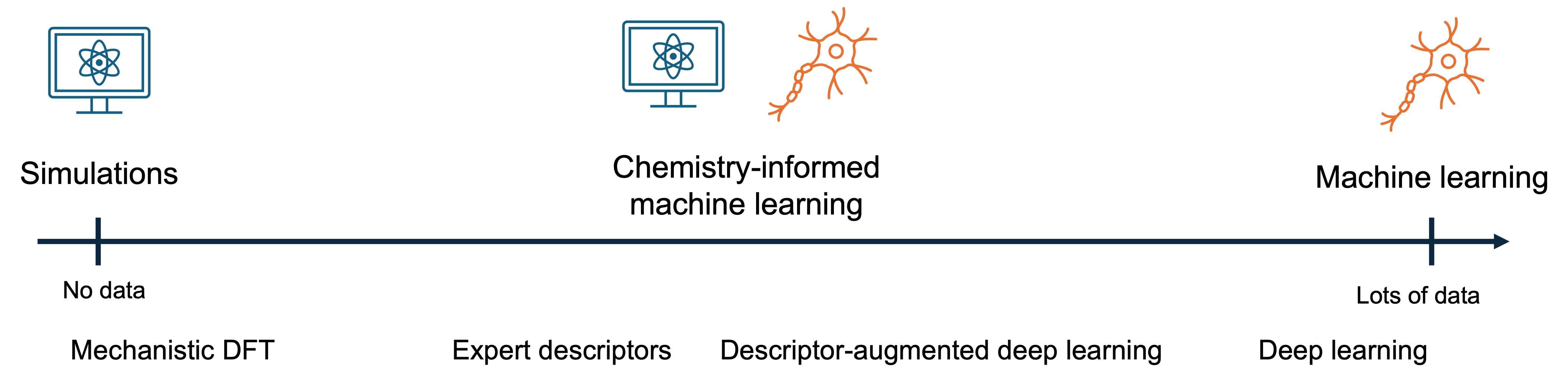
The choice of representation depends on the amount of data available, the complexity of the problem, and whether interpretability matters.
{width="100%"}
Rules of thumb:
- **Very small datasets (\< 50)**: use expert descriptors (Sterimol, Hammett, computed LogP). These inject chemical knowledge and keep the model simple enough to avoid overfitting.
- **Small to medium datasets (50--500)**: fingerprints with classical ML models (random forest, gradient boosting) work well. Augment with computed descriptors.
- **Large datasets (500+)**: deep learning approaches (graph neural networks, transformers) can learn optimal representations directly from the molecular structure.
- **For interpretability**: simple descriptors and linear models are preferred. Fingerprints with feature importance can also provide insight.
- **Descriptor-augmented deep learning** is a hybrid approach that feeds expert descriptors alongside learned representations into a neural network, combining the best of both worlds.
## Summary
There is no best representation, only a trade-off between how much chemistry is encoded and what that costs — in computation, in the data needed to use it, and in how far the result generalizes. If you have a small dataset, expert descriptors are usually the way to go; if you have a large dataset, learned representations can extract more information. A whole spectrum of representations exists between these extremes, and the right choice depends on the problem at hand.