9  Graph Models

In the cheminformatics chapter we converted molecules into machine-readable representations by hand: SMILES strings, fingerprints, and expert descriptors. Each of these is a fixed recipe that we design before the model ever sees the data. But there is a more natural mathematical structure waiting to be used: the Lewis structure we draw for a molecule is a graph. Atoms are nodes, bonds are edges. Rather than hand-designing descriptors, we can let a neural network operate directly on this graph and learn the representation that best predicts the property we care about.

This idea of representation learning instead of fixed expert descriptors (Yang et al. 2019) is what separates graph neural networks (GNNs) from the classical workflows. This chapter builds GNNs from the ground up: first the data structures (adjacency, node features, edge features), then the core message-passing machinery, then the inductive biases and known failure modes, and finally the extension to 3D structures and neural-network potentials that can replace expensive quantum calculations.

9.1 Molecules as graphs

A graph \(G = (\mathcal{V}, \mathcal{E})\) is a collection of vertices (nodes) \(\mathcal{V}\) and edges \(\mathcal{E}\) connecting them. Graphs can be directed (edges have a direction, like arrows) or undirected, and both nodes and edges can carry labels. A friendship network, a citation graph, and a road map are all graphs.

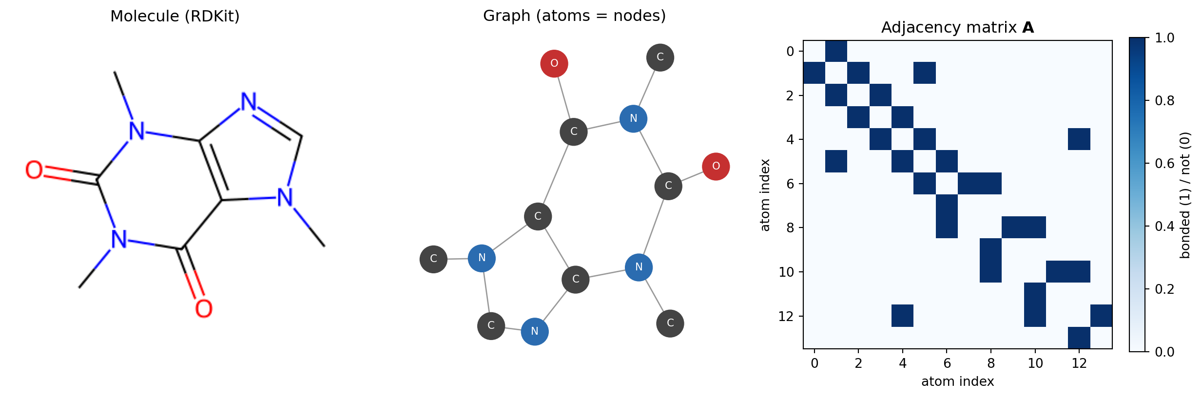
A molecule is naturally a node- and edge-labeled undirected graph: atoms are the nodes (labeled by element, charge, hybridization, …), bonds are the undirected edges (labeled by bond order). To feed this graph to a neural network we need numerical data structures:

• Adjacency matrix \(\mathbf{A}\) — an \(N \times N\) binary matrix (\(N\) = number of atoms) encoding connectivity. \(A_{ij} = 1\) if atoms \(i\) and \(j\) are bonded, \(0\) otherwise. Because molecular bonds are undirected, \(\mathbf{A}\) is symmetric.
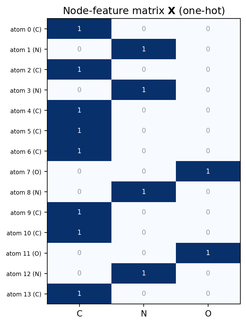
• Node-feature matrix \(\mathbf{X}\) — one row per atom. Features typically include a one-hot encoding of the atom type (C, N, O, …) plus extra descriptors such as degree, formal charge, and aromaticity.
• Edge-feature matrix \(\mathbf{X}_e\) — one row per bond, typically a one-hot encoding of the bond type (single, double, triple, aromatic).

Almost all of these labels are one-hot encoded so that the network treats categories (e.g. “carbon” vs “nitrogen”) as distinct dimensions rather than as an ordinal scale. This means the network doesn’t get any prior knowledge on element similarity or periodic table relations. Like in chemoinformatics, it’s possible to work with all-atom chemical graph or with chemical graph with implicit hydrogens.

from rdkit import Chem
from rdkit.Chem import Draw
import numpy as np
import networkx as nx
import matplotlib.pyplot as plt

np.random.seed(0)

mol = Chem.MolFromSmiles("Cn1cnc2c1c(=O)n(C)c(=O)n2C")  # Caffeine
A = Chem.GetAdjacencyMatrix(mol)
symbols = [atom.GetSymbol() for atom in mol.GetAtoms()]

# RDKit drawing -> PIL image
rdkit_img = Draw.MolToImage(mol, size=(300, 300))

# networkx graph
G = nx.from_numpy_array(np.array(A))
color_map = {"C": "#444444", "N": "#2b6cb0", "O": "#c53030"}
node_colors = [color_map.get(s, "#888888") for s in symbols]

fig, axes = plt.subplots(1, 3, figsize=(13, 4.2))

axes[0].imshow(rdkit_img)
axes[0].axis("off")
axes[0].set_title("Molecule (RDKit)")

pos = nx.spring_layout(G, seed=1)
nx.draw(G, pos, ax=axes[1], node_color=node_colors, with_labels=True,
        labels={i: symbols[i] for i in range(len(symbols))},
        font_color="white", node_size=420, font_size=8, edge_color="#999999")
axes[1].set_title("Graph (atoms = nodes)")

im = axes[2].imshow(A, cmap="Blues", interpolation="nearest")
axes[2].set_title("Adjacency matrix $\\mathbf{A}$")
axes[2].set_xlabel("atom index")
axes[2].set_ylabel("atom index")
plt.colorbar(im, ax=axes[2], fraction=0.046, label="bonded (1) / not (0)")

plt.tight_layout()
plt.show()

Figure 9.1: Caffeine as a graph: the molecule (left), its connectivity drawn with networkx (center), and its binary adjacency matrix as a heatmap (right). The adjacency matrix is symmetric because bonds are undirected.

The node-feature matrix is built by one-hot encoding. If we restrict ourselves to the elements present in caffeine, each atom becomes a short binary vector:

import numpy as np
import matplotlib.pyplot as plt

elements = ["C", "N", "O"]
onehot = np.array([[1 if s == e else 0 for e in elements] for s in symbols])

fig, ax = plt.subplots(figsize=(4.2, 5.5))
ax.imshow(onehot, cmap="Blues", aspect="auto")
ax.set_xticks(range(len(elements)))
ax.set_xticklabels(elements)
ax.set_yticks(range(len(symbols)))
ax.set_yticklabels([f"atom {i} ({s})" for i, s in enumerate(symbols)], fontsize=7)
ax.set_title("Node-feature matrix $\\mathbf{X}$ (one-hot)")
for i in range(onehot.shape[0]):
    for j in range(onehot.shape[1]):
        ax.text(
            j,
            i,
            onehot[i, j],
            ha="center",
            va="center",
            color="white" if onehot[i, j] else "#999999",
            fontsize=8,
        )
plt.tight_layout()
plt.show()

Figure 9.2: One-hot node features for the atoms of caffeine over the columns [C, N, O]. Each atom is a row; a 1 marks its element.

So a molecule is fully described by the triple \((\mathbf{A}, \mathbf{X}, \mathbf{X}_e)\). The next question is: how do we build a neural network that consumes these and produces a property prediction?

TipUnderstanding check

Suppose the node features are one-hot encoded atom types over the elements [C, N, O, F], and the edge features are one-hot encoded bond types over [single, double, triple, aromatic]. What are the shapes of \(\mathbf{A}\), \(\mathbf{X}\), and \(\mathbf{X}_e\) for the caffeine example shown above?

NoteShow solution

Caffeine has 14 atoms (8 C, 4 N, 2 O) and 15 bonds (10 aromatic, 3 single, 2 double), so:

• \(\mathbf{A}\) is \(14 \times 14\) — one row and column per atom (and symmetric, since bonds are undirected).
• \(\mathbf{X}\) is \(14 \times 4\) — one row per atom, with a one-hot atom-type encoding over the four columns [C, N, O, F]. (Caffeine contains no fluorine, so the F column is all zeros — the width is fixed by the set of element types chosen in advance, not by which elements happen to appear in this molecule.)
• \(\mathbf{X}_e\) is \(15 \times 4\) — one row per bond, with a one-hot bond-type encoding over [single, double, triple, aromatic].

The row counts (\(14\), \(14\), \(15\)) come straight from the molecule; the column counts (\(4\) and \(4\)) are the sizes of the chosen atom-type and bond-type sets. If edges were instead stored as directed pairs (as many message-passing implementations do), \(\mathbf{X}_e\) would have \(2 \times 15 = 30\) rows.

9.2 From graph convolutions to message passing

9.2.1 Graph convolutions

The central operation of a GNN is the graph convolution: update each node by mixing its own features with those of its neighbors. The simplest form, written per node \(i\), is

\[ \mathbf{x}'_i = \mathbf{x}_i \mathbf{W}_1 + \sum_{j \in N(i)} \mathbf{x}_j \mathbf{W}_2 + \mathbf{b} \]

where \(\mathbf{x}_i\) is the current feature vector of node \(i\), \(N(i)\) is the set of its neighbors, and \(\mathbf{W}_1\), \(\mathbf{W}_2\), \(\mathbf{b}\) are learnable weight matrices and a bias. The first term keeps the node’s own information; the second term aggregates information from its bonded neighbors.

The same operation can be written for the whole node matrix at once:

\[ \mathbf{X}' = \mathbf{X}\mathbf{W}_1 + \mathbf{A}\mathbf{X}\mathbf{W}_2 + \mathbf{b} \]

Here the multiplication by the adjacency matrix \(\mathbf{A}\) is what selects neighbors: row \(i\) of \(\mathbf{A}\mathbf{X}\) is exactly \(\sum_{j \in N(i)} \mathbf{x}_j\), the sum over the neighbors of \(i\). This compact matrix form is why GNNs run efficiently on hardware built for matrix multiplication.

9.2.2 Stacking convolutions grows the receptive field

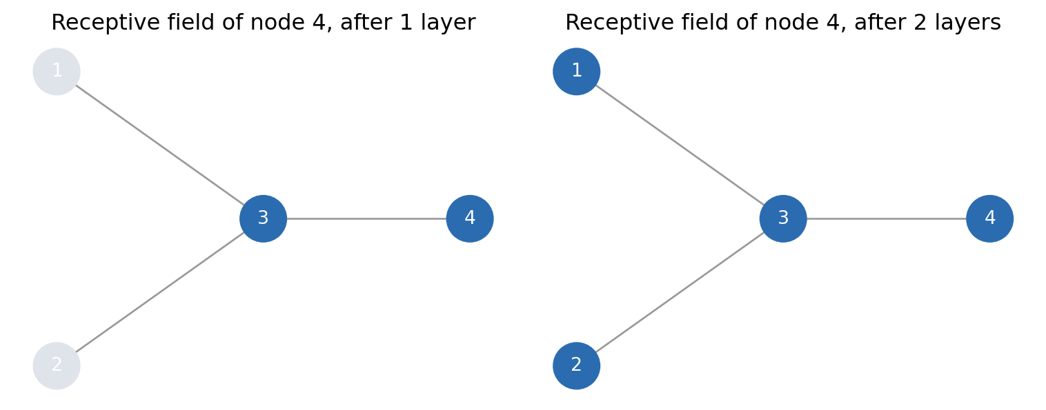
A single convolution only lets a node “see” its immediate, one-bond neighbors. The power comes from stacking layers. After the first convolution, node \(i\)’s embedding already contains information from its 1-hop neighbors. After the second convolution it mixes in their neighbors, so it now sees 2-hop neighbors, and so on. Formally, take the small 4-node graph in Figure 9.3, in which node \(3\) is bonded to nodes \(1\), \(2\), and \(4\), while node \(4\) is bonded only to node \(3\). The first convolution applied to node \(4\) reaches node \(3\) and through it nodes \(1\) and \(2\) that are two bonds away. Each layer expands the receptive field by one hop.

import networkx as nx
import matplotlib.pyplot as plt

G = nx.Graph([(3, 1), (3, 2), (3, 4)])
pos = {1: (0, 1), 2: (0, -1), 3: (1, 0), 4: (2, 0)}
seen = {"after 1 layer": {4, 3}, "after 2 layers": {4, 3, 1, 2}}

fig, axes = plt.subplots(1, 2, figsize=(8, 3.2))
for ax, (title, reached) in zip(axes, seen.items()):
    nx.draw_networkx_edges(G, pos, ax=ax, edge_color="#999999")
    nx.draw_networkx_nodes(G, pos, ax=ax, node_size=620,
                           node_color=["#2b6cb0" if n in reached else "#dfe3ea"
                                       for n in G.nodes])
    nx.draw_networkx_labels(G, pos, ax=ax, font_size=10,
                            font_color="white" if reached else "black")
    ax.set_title(f"Receptive field of node 4, {title}")
    ax.axis("off")
plt.tight_layout()
plt.show()

Figure 9.3: Growth of the receptive field of node 4 in a 4-node graph. After one layer (left) node 4 has seen only its direct neighbour, node 3. After two layers (right) the information from nodes 1 and 2 has reached it through node 3.

This is the locality inductive bias: information spreads gradually, neighbor by neighbor. Note that the weight matrices \(\mathbf{W}_1^{(t)}, \mathbf{W}_2^{(t)}\) can be different for each layer \(t\).

9.2.3 The message-passing formalism (MPNN)

The graph convolution above is one special case of a much more general and flexible framework: the message-passing neural network (MPNN). Every layer \(t\) performs two steps.

Step 1 — message (aggregate over neighbors):

\[ \mathbf{m}_i = \sum_{j \in N(i)} M_t\!\left(\mathbf{h}_i^{(t)},\, \mathbf{h}_j^{(t)},\, \mathbf{e}_{ij}\right) \]

Step 2 — update (combine the node’s state with the incoming message):

\[ \mathbf{h}_i^{(t+1)} = U_t\!\left(\mathbf{h}_i^{(t)},\, \mathbf{m}_i\right) \]

The pieces are:

• \(\mathbf{h}_i^{(t)}\) — the hidden state of node \(i\) at layer \(t\) (its current feature vector). The very first layer is initialized with the input features, \(\mathbf{h}_i^{(0)} = \mathbf{x}_i\).
• \(M_t\) — the message function, which decides how a neighbor \(j\) contributes to node \(i\).
• \(U_t\) — the update function, which folds the aggregated message back into the node.
• \(\mathbf{e}_{ij}\) — the edge features between \(i\) and \(j\) (e.g. the bond type, or in 3D the interatomic distance).
• \(t\) — the layer (convolution) index.

The simple graph convolution is recovered by choosing \(M_t(\mathbf{h}_i, \mathbf{h}_j, \mathbf{e}_{ij}) = \mathbf{h}_j \mathbf{W}_2\) and \(U_t(\mathbf{h}_i, \mathbf{m}_i) = \mathbf{h}_i \mathbf{W}_1 + \mathbf{m}_i + \mathbf{b}\):

\[ \mathbf{h}_i^{(t+1)} = \mathbf{h}_i^{(t)}\mathbf{W}_1 + \sum_{j\in N(i)}\mathbf{h}_j^{(t)}\mathbf{W}_2 + \mathbf{b}. \]

Different choices of \(M_t\) and \(U_t\) give different GNN architectures — graph attention networks, the directed-MPNN behind Chemprop, SchNet (which we will meet below), and many more. The message-passing template is the unifying language for all of them.

9.2.4 Readout / pooling → prediction

After \(T\) message-passing layers (where \(T\) is a hyperparameter, not to be confused with the number of atoms \(N\)) we have a learned vector for every atom. But a molecule can have any number of atoms, and the atom numbering is arbitrary — so we cannot just feed these vectors into a normal neural network. We need a readout (or pooling) step that collapses the variable-size set of node vectors into a single fixed-length graph vector:

\[ \mathbf{h}_{G} = \bigoplus_{i \in \mathcal{V}} \mathbf{h}_i^{(T)}, \qquad \bigoplus \in \{\text{sum},\ \text{mean},\ \text{max}\}. \]

This graph vector then passes through one or more fully connected layers to the final prediction — a linear output for regression, or a softmax/sigmoid for classification.

Pooling is doing two crucial jobs at once. First, it lets the model handle molecules of different sizes, because the output length no longer depends on \(N\). Second, because sum/mean/max do not care about the order of their inputs, pooling makes the graph-level output permutation invariant — the prediction is the same no matter how we number the atoms.

9.2.5 Interactive: message passing & the receptive field

The widget below shows a small fixed graph. Use the slider to set the number of message-passing layers, and watch both the receptive field (left panel) and the node values (right panel) change.

#| '!! shinylive warning !!': |
#|   shinylive does not work in self-contained HTML documents.
#|   Please set `embed-resources: false` in your metadata.
#| standalone: true
#| viewerHeight: 560

from shiny import App, render, ui, reactive
import matplotlib.pyplot as plt
import matplotlib
import numpy as np

matplotlib.rcParams.update({
    "font.family": "serif",
    "figure.facecolor": "#fafaf7",
    "axes.facecolor": "#fafaf7",
})

# Fixed 8-node graph (hand-coded)
pos = np.array([
    [0.0, 1.0],   # 0  source
    [1.0, 1.8],   # 1
    [1.0, 0.2],   # 2
    [2.2, 1.0],   # 3
    [3.4, 1.7],   # 4
    [3.4, 0.3],   # 5
    [4.6, 1.0],   # 6
    [2.2, 2.6],   # 7
])
edges = [(0, 1), (0, 2), (1, 3), (2, 3), (3, 4), (3, 5),
         (4, 6), (5, 6), (1, 7), (7, 4)]
N = pos.shape[0]
A = np.zeros((N, N))
for i, j in edges:
    A[i, j] = 1
    A[j, i] = 1
SOURCE = 0

# Initial scalar feature per node (distinct values)
feat0 = np.array([1.0, 0.2, 0.8, 0.5, 0.1, 0.9, 0.3, 0.7])

app_ui = ui.page_fluid(
    ui.input_slider("layers", "Message-passing layers", min=0, max=5, value=1, step=1),
    ui.output_plot("mp_plot"),
)

def server(input, output, session):
    @output
    @render.plot
    def mp_plot():
        L = input.layers()

        # Reachable set after L hops via repeated adjacency multiplication
        reach = np.zeros(N)
        reach[SOURCE] = 1.0
        AplusI = A + np.eye(N)
        for _ in range(L):
            reach = (AplusI @ reach > 0).astype(float)
        reached = reach > 0

        # Oversmoothing: repeated neighbor averaging (row-normalized A+I)
        deg = AplusI.sum(axis=1, keepdims=True)
        P = AplusI / deg
        feat = feat0.copy()
        for _ in range(L):
            feat = P @ feat

        fig, axes = plt.subplots(1, 2, figsize=(9, 4.6))

        # --- Left: receptive field ---
        ax = axes[0]
        for i, j in edges:
            ax.plot([pos[i, 0], pos[j, 0]], [pos[i, 1], pos[j, 1]],
                    color="#cccccc", lw=1.5, zorder=1)
        colors = ["#2b6cb0" if reached[k] else "#dddddd" for k in range(N)]
        ax.scatter(pos[:, 0], pos[:, 1], s=600, c=colors, zorder=2,
                   edgecolors="white", linewidths=2)
        ax.scatter(pos[SOURCE, 0], pos[SOURCE, 1], s=900, facecolors="none",
                   edgecolors="#c53030", linewidths=3, zorder=3)
        for k in range(N):
            ax.text(pos[k, 0], pos[k, 1], str(k), ha="center", va="center",
                    color="white" if reached[k] else "#888888",
                    fontsize=11, fontweight="bold", zorder=4)
        ax.set_title("Receptive field after %d layers\n%d of %d nodes reached"
                     % (L, int(reached.sum()), N), fontsize=11)
        ax.set_xlim(-0.7, 5.3)
        ax.set_ylim(-0.5, 3.2)
        ax.axis("off")

        # --- Right: oversmoothing ---
        ax2 = axes[1]
        for i, j in edges:
            ax2.plot([pos[i, 0], pos[j, 0]], [pos[i, 1], pos[j, 1]],
                     color="#cccccc", lw=1.5, zorder=1)
        sc = ax2.scatter(pos[:, 0], pos[:, 1], s=600, c=feat, cmap="viridis",
                         vmin=0, vmax=1, zorder=2, edgecolors="white", linewidths=2)
        for k in range(N):
            ax2.text(pos[k, 0], pos[k, 1], "%.2f" % feat[k], ha="center", va="center",
                     color="white", fontsize=8, fontweight="bold", zorder=4)
        spread = feat.max() - feat.min()
        ax2.set_title("Oversmoothing after %d layers\nvalue spread = %.3f"
                      % (L, spread), fontsize=11)
        ax2.set_xlim(-0.7, 5.3)
        ax2.set_ylim(-0.5, 3.2)
        ax2.axis("off")
        fig.colorbar(sc, ax=ax2, fraction=0.046, label="node value")

        fig.tight_layout()
        return fig

app = App(app_ui, server)

NoteWhat to notice

Increasing the number of layers does two things at once:

• The receptive field grows ring by ring (left panel), starting from the highlighted source node, until every node is reached — this is why deeper GNNs can capture longer-range structure.
• The node values converge (right panel): their spread shrinks toward zero. This is oversmoothing.

To make oversmoothing transparent, the widget uses the bare-minimum graph convolution: each node holds a single scalar feature, so the weight matrices \(\mathbf{W}_1, \mathbf{W}_2\) collapse to plain numbers that we fix to \(1\) (no learnable transform, no bias), and the aggregation is a simple average — each layer replaces a node’s value by the mean of itself and its bonded neighbors (the self-loop comes from \(\mathbf{A} + \mathbf{I}\)). After enough layers every node reaches nearly the same value, washing out all local information.

So you cannot just keep stacking layers to reach longer range without destroying the local detail that made the representation useful. The same tendency persists in real, deeper GNNs with learnable weights and high-dimensional features — it is simply less dramatic there, since the learnable transforms (and tricks such as residual connections) can partly counteract the smoothing. It remains a key reason GNNs we have to resort to more advanced tricks to make deep GNNs work well.

9.3 Inductive biases of GNNs

Why are GNNs so data-efficient for molecules compared with, say, treating a molecule as an unordered bag of atoms? The answer is the inductive biases baked into their architecture — assumptions about the structure of the problem that the model does not have to learn from scratch.

• Permutation equivariance / invariance. The atoms in a molecule have no canonical ordering; atom “1” could equally have been numbered “7”. Message passing is permutation-equivariant: relabel the atoms and the per-node outputs come along with exactly the same relabeling, with no change in the underlying computation. The pooling step then makes the graph-level output permutation-invariant: the prediction is identical regardless of numbering. A model that did not have this property would have to waste data learning that all \(N!\) orderings of the same molecule are equivalent.
• Locality. Information spreads gradually, one bond at a time. This matches chemical intuition: an atom’s behavior is dominated by its local environment, with longer-range effects entering more slowly. The locality bias steers the model toward physically reasonable functions and away from spurious global correlations.

The unconstrained model to compare against is a plain feed-forward network, which needs a fixed-size input: fix a maximum atom count \(N_{\max}\), order the atoms somehow, concatenate their feature vectors and zero-pad to \(N_{\max}\), with the adjacency matrix flattened and padded alongside.

Because the ordering is arbitrary but fixed, this network learns weights tied to positions in the vector rather than to atoms, so permuting the atoms gives a different input for the same molecule; and every input position is connected alike, so locality has to be learned too. Both must come from data — typically via permutation augmentation — whereas the GNN gets them from its architecture.

9.4 Known limitations

WarningGNNs are powerful but have real failure modes

• Oversmoothing. Stacking too many message-passing layers drives all node representations toward the same value (you saw this in the interactive widget). The useful local distinctions between atoms get washed out, and performance degrades rather than improves with very deep networks.

• Oversquashing. The receptive field grows exponentially with depth, but the messages flowing along the graph must pass through fixed-width node states at every step. Information from an exponentially large neighborhood gets “squashed” through these narrow channels, so long-range dependencies are hard to capture even when the receptive field nominally covers them.

• Data-hungry and poor extrapolation. A GNN that learns its representation from scratch typically needs a lot of training data, and it extrapolates poorly outside the region of chemical space it was trained on. With little data, expert descriptors + classical ML can win — exactly the trade-off discussed in the cheminformatics and physics-based chapters. Choosing between learned and fixed representations is fundamentally a question of how much data you have.

TipFurther reading

Two excellent, highly visual introductions to graph neural networks are the Distill articles A Gentle Introduction to Graph Neural Networks (Sanchez-Lengeling et al. 2021) and Understanding Convolutions on Graphs (Daigavane et al. 2021). Both are interactive and build strong intuition for the message-passing machinery and design choices covered in this chapter.

9.5 Beyond the 2D chemical graph

So far our edges have been chemical bonds. But the message-passing machinery does not require that. We can build edges in other ways, and crucially we can move from 2D connectivity to full 3D geometry.

9.5.1 Chemical graph vs. fully connected graph

• The chemical (bond) graph uses bonds as edges — this is the molecular graph we have used all along.
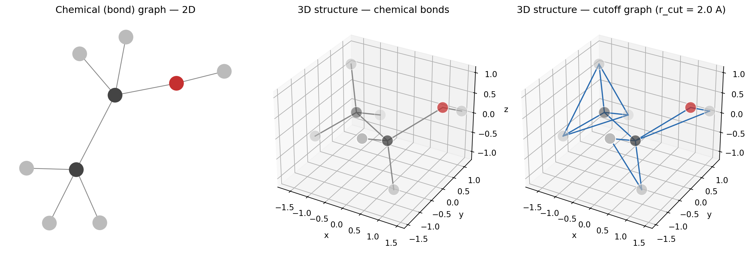
• A distance-cutoff graph instead connects every pair of atoms that lie within some cutoff radius \(r_{\text{cut}}\), whether or not they are formally bonded. This captures non-bonded interactions (steric clashes, hydrogen bonds, electrostatics) that the bond graph misses entirely, and it is the natural choice for 3D models. In the limit \(r_{\text{cut}} \to \infty\) this becomes the fully connected graph in which every atom sees every other. This is precisely the setting of the transformer: self-attention is message passing on a fully connected graph, with the attention weights acting as learned, input-dependent edge importances — a viewpoint developed by Veličković (2023), who argues that transformers are a special case of graph neural networks.

9.5.2 2D vs. 3D graphs (point clouds)

A 3D model takes the atomic coordinates — a point cloud \(\{\mathbf{r}_1, \dots, \mathbf{r}_N\}\) — and constructs edges from the interatomic distances, connecting atoms within the cutoff. The geometry, not just the topology, becomes part of the input.

from rdkit import Chem
from rdkit.Chem import AllChem
import numpy as np
import networkx as nx
import matplotlib.pyplot as plt

mol = Chem.MolFromSmiles("CCO")
mol = Chem.AddHs(mol)
AllChem.EmbedMolecule(mol, randomSeed=42)
AllChem.MMFFOptimizeMolecule(mol)
conf = mol.GetConformer()
coords = np.array([list(conf.GetAtomPosition(i)) for i in range(mol.GetNumAtoms())])
syms = [a.GetSymbol() for a in mol.GetAtoms()]
cmap = {"C": "#444444", "O": "#c53030", "H": "#bbbbbb"}
ncol = [cmap[s] for s in syms]
N = mol.GetNumAtoms()

# Chemical bonds, and the extra edges a distance cutoff adds
bond_edges = [(b.GetBeginAtomIdx(), b.GetEndAtomIdx()) for b in mol.GetBonds()]
cutoff = 2.0
cut_edges = [(i, j) for i in range(N) for j in range(i + 1, N)
             if np.linalg.norm(coords[i] - coords[j]) <= cutoff]

fig = plt.figure(figsize=(13, 4.4))

# --- Left: 2D chemical (bond) graph ---
ax1 = fig.add_subplot(1, 3, 1)
G_bond = nx.Graph()
G_bond.add_nodes_from(range(N))
G_bond.add_edges_from(bond_edges)
pos2d = nx.spring_layout(G_bond, seed=2)
nx.draw(G_bond, pos2d, ax=ax1, node_color=ncol, node_size=300,
        edge_color="#888888", with_labels=False)
ax1.set_title("Chemical (bond) graph — 2D")

def draw_3d(ax, edges, edge_color, title):
    ax.scatter(coords[:, 0], coords[:, 1], coords[:, 2],
               c=ncol, s=200, edgecolors="white", linewidths=1)
    for i, j in edges:
        ax.plot(*zip(coords[i], coords[j]), color=edge_color, lw=1.5)
    ax.set_title(title)
    ax.set_xlabel("x")
    ax.set_ylabel("y")
    ax.set_zlabel("z")

# --- Center: 3D with chemical bonds ---
ax2 = fig.add_subplot(1, 3, 2, projection="3d")
draw_3d(ax2, bond_edges, "#888888", "3D structure — chemical bonds")

# --- Right: 3D with distance-cutoff edges ---
ax3 = fig.add_subplot(1, 3, 3, projection="3d")
draw_3d(ax3, cut_edges, "#2b6cb0", "3D structure — cutoff graph (r_cut = %.1f A)" % cutoff)

plt.tight_layout()
plt.show()

Figure 9.4: Three views of the same molecule (ethanol). Left: the chemical bond graph (2D, topological). Center: the 3D structure with the same chemical bonds as edges. Right: the 3D structure with a distance-cutoff graph (all atom pairs within 2.0 A connected, which adds non-bonded contacts on top of the bonds).

9.5.3 Invariance vs. equivariance

Moving to 3D raises a subtle but essential requirement. The prediction must respect the symmetries of physical space. Two cases (Isert et al. 2023):

• A scalar property such as the energy must be invariant under rotation and translation: rotating the whole molecule does not change its energy, so the model’s output must not change either.
• A vector property such as the dipole moment must be equivariant: rotate the molecule and the dipole vector must rotate with it by the same amount.

3D GNNs achieve these guarantees by construction:

• Permutation invariance comes from pooling (as in 2D).
• Rotation/translation invariance comes from using interatomic distances rather than raw coordinates, since distances are unchanged by rigid motions (the same trick behind the Coulomb matrix representation from the physics-based chapter).
• Equivariance for vector outputs comes from additionally encoding angular information so the network can track orientation.

9.5.4 Interactive: invariance vs. equivariance

Rotate the small molecule below with the slider. The predicted scalar “energy” stays constant (invariant) no matter how you rotate it, while the “dipole” arrow rotates together with the molecule (equivariant). This is exactly the behavior a correct 3D model must reproduce.

#| '!! shinylive warning !!': |
#|   shinylive does not work in self-contained HTML documents.
#|   Please set `embed-resources: false` in your metadata.
#| standalone: true
#| viewerHeight: 560

from shiny import App, render, ui, reactive
import matplotlib.pyplot as plt
import matplotlib
import numpy as np

matplotlib.rcParams.update(
    {
        "font.family": "serif",
        "figure.facecolor": "#fafaf7",
        "axes.facecolor": "#fafaf7",
    }
)

# Hand-coded formaldehyde (H2C=O): central carbon, double-bonded oxygen, two H (planar)
atoms0 = np.array(
    [
        [0.0, 0.0],  # C (center)
        [1.0, 0.0],  # O (double bond)
        [-0.5, 0.9],  # H
        [-0.5, -0.9],  # H
    ]
)
bonds = [(0, 1), (0, 2), (0, 3)]
double_bonds = {(0, 1)}  # the C=O bond
atom_colors = ["#222222", "#c53030", "#bbbbbb", "#bbbbbb"]  # C black, O red, H grey

# Dipole vector in the molecule frame (along C=O), plus a perpendicular offset so
# the arrow is drawn beside the double bond instead of on top of it.
dipole0 = np.array([0.9, 0.0])
dipole_offset0 = np.array([0.0, -0.4])
ENERGY = 4.73  # constant scalar property

app_ui = ui.page_fluid(
    ui.output_plot("eq_plot"),
    ui.input_slider(
        "angle", "Rotation angle (degrees)", min=0, max=360, value=0, step=5
    ),
)


def server(input, output, session):
    @output
    @render.plot
    def eq_plot():
        theta = np.deg2rad(input.angle())
        R = np.array([[np.cos(theta), -np.sin(theta)], [np.sin(theta), np.cos(theta)]])
        atoms = atoms0 @ R.T

        fig, ax = plt.subplots(figsize=(7, 6))
        ax.set_xlim(-2.2, 2.6)
        ax.set_ylim(-2.2, 2.2)
        ax.set_aspect("equal")
        ax.axhline(0, color="#dddddd", lw=0.8)
        ax.axvline(0, color="#dddddd", lw=0.8)

        # bonds (the C=O is drawn as a double line)
        for i, j in bonds:
            p, q = atoms[i], atoms[j]
            if (i, j) in double_bonds:
                d = q - p
                n = np.array([-d[1], d[0]])
                n = n / np.linalg.norm(n) * 0.07
                for s in (1, -1):
                    ax.plot(
                        [p[0] + s * n[0], q[0] + s * n[0]],
                        [p[1] + s * n[1], q[1] + s * n[1]],
                        color="#999999",
                        lw=2.5,
                        zorder=1,
                    )
            else:
                ax.plot([p[0], q[0]], [p[1], q[1]], color="#999999", lw=2.5, zorder=1)
        # atoms
        ax.scatter(
            atoms[:, 0],
            atoms[:, 1],
            s=700,
            c=atom_colors,
            edgecolors="white",
            linewidths=2,
            zorder=2,
        )

        # dipole arrow (equivariant), offset beside the C=O bond so it doesn't overlap it
        start = R @ dipole_offset0
        end = R @ (dipole0 + dipole_offset0)
        ax.annotate(
            "",
            xy=(end[0], end[1]),
            xytext=(start[0], start[1]),
            arrowprops=dict(arrowstyle="-|>", color="#805ad5", lw=3),
            zorder=3,
        )
        txt = R @ (dipole0 + dipole_offset0 + np.array([0.2, -0.4]))
        ax.text(
            txt[0],
            txt[1],
            "dipole\n(equivariant)",
            color="#805ad5",
            fontsize=10,
            fontweight="bold",
            ha="center",
            va="center",
        )

        # invariant scalar
        ax.text(
            -2.0,
            1.9,
            "Energy = %.2f  (invariant)" % ENERGY,
            fontsize=12,
            fontweight="bold",
            color="#c53030",
        )

        ax.set_title(
            "Rotate the molecule:\nenergy stays fixed, dipole rotates with it",
            fontsize=12,
        )
        ax.axis("off")
        fig.tight_layout(rect=[0, 0, 1, 0.92])
        return fig


app = App(app_ui, server)

Notice that the scalar energy is printed unchanged for every rotation angle (invariant), while the dipole arrow’s direction tracks the molecule (equivariant). A model that let the energy drift as you rotated would be physically wrong, and one whose dipole pointed in a fixed lab direction regardless of the molecule would be equally wrong.

9.6 Neural-network (machine-learning) potentials

The biggest payoff of 3D GNNs is the neural-network potential (NNP, also called a machine-learning interatomic potential, MLIP). The idea: train a GNN to predict the energy directly from the 3D structure, bypassing the expensive self-consistent-field (SCF) / DFT calculation. Once trained, evaluation is dramatically cheaper — the lecture quotes roughly 10,000 s for a quantum simulation vs. ~0.01 s for the GNN, a factor of about \(10^6\).

This unlocks fast molecular dynamics at near-quantum accuracy. Crucially, the predicted energy is differentiable, so:

• Forces come from automatic differentiation of the energy with respect to coordinates, \(\mathbf{F}_i = -\partial E / \partial \mathbf{r}_i\).¹
• Vibrational frequencies come from second derivatives.

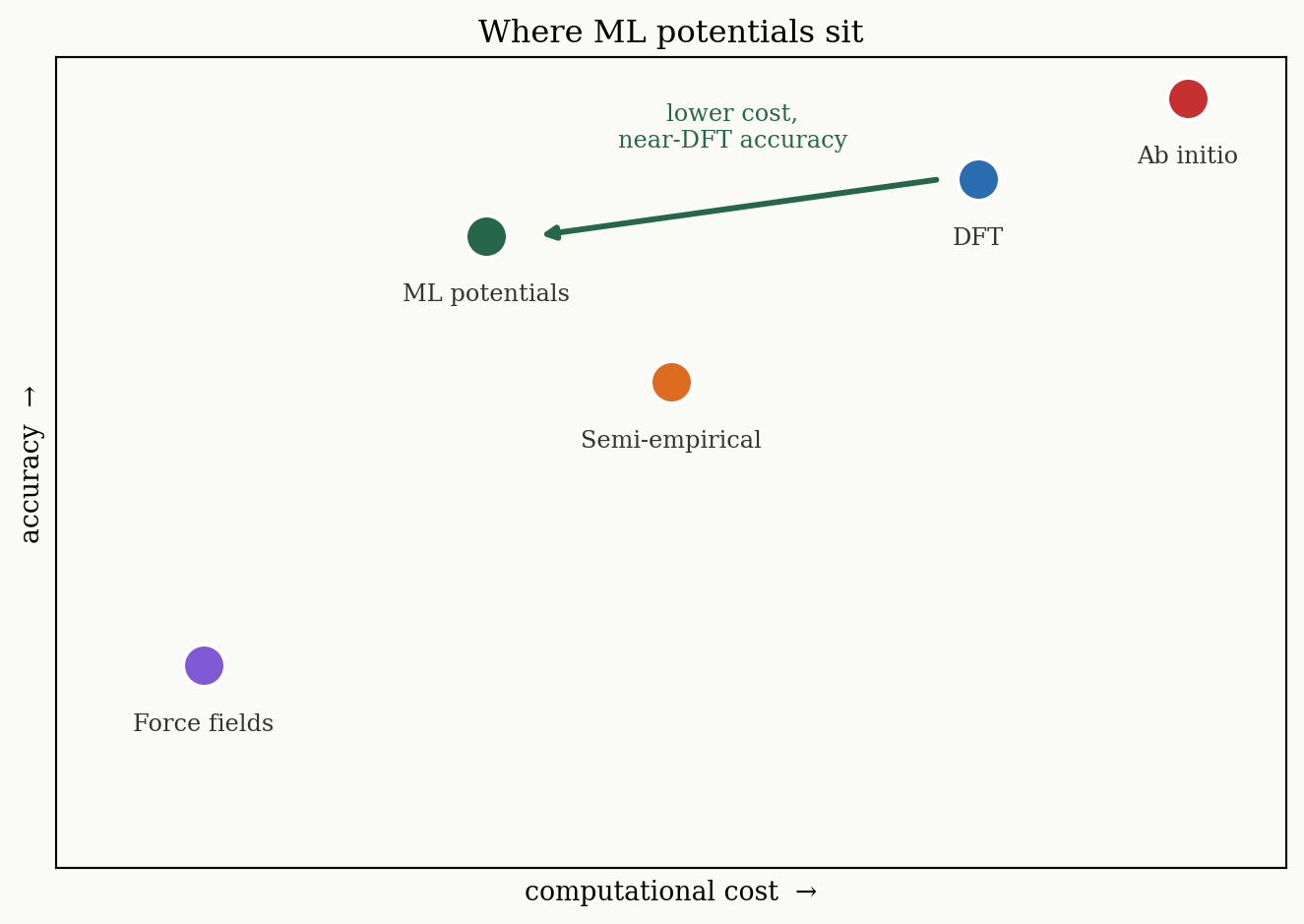
On a cost-vs-accuracy spectrum, NNPs sit between cheap classical force fields and expensive DFT/ab-initio methods. Example models include ANI (ANI-1ccx, ANI-2x), MACE-OFF, SchNet, PhysNet, and UMA family of models.

9.6.1 SchNet: distances as edge features

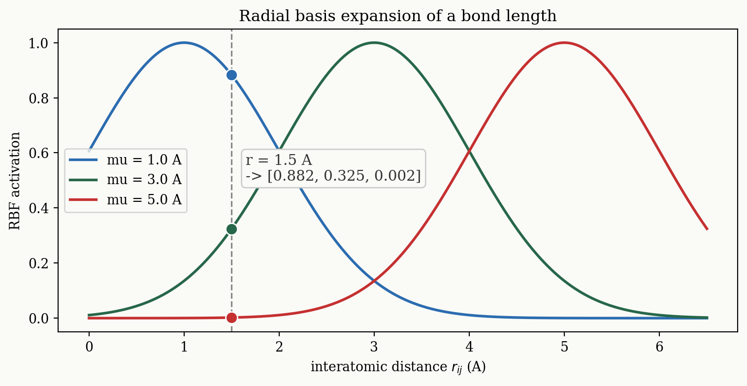
SchNet uses the interatomic distance \(r_{ij}\) as the edge feature, but feeding a raw distance into a network works poorly. Instead it expands the distance in a radial basis of Gaussians:

\[ \mathbf{e}_{ij} = \exp\!\left(-\gamma\,(r_{ij} - \mu)^2\right) \]

with a set of centers \(\mu\) spread across the relevant distance range. A single bond length is thus turned into a smooth vector of activations — one per Gaussian — which gives the network a soft, differentiable encoding of distance that feeds into the message function.

import numpy as np
import matplotlib.pyplot as plt

np.random.seed(0)
plt.rcParams.update({"font.family": "serif",
                     "figure.facecolor": "#fafaf7",
                     "axes.facecolor": "#fafaf7"})

centers = np.array([1.0, 3.0, 5.0])
gamma = 0.5
r = np.linspace(0, 6.5, 400)
r_query = 1.5

fig, ax = plt.subplots(figsize=(8, 4.2))
colors = ["#2b6cb0", "#276749", "#c53030"]
activations = []
for mu, c in zip(centers, colors):
    y = np.exp(-gamma * (r - mu) ** 2)
    ax.plot(r, y, color=c, lw=2, label="mu = %.1f A" % mu)
    a = np.exp(-gamma * (r_query - mu) ** 2)
    activations.append(a)
    ax.scatter([r_query], [a], color=c, s=80, zorder=5, edgecolors="white")

ax.axvline(r_query, color="#888888", ls="--", lw=1.2)
ax.set_xlabel("interatomic distance $r_{ij}$ (A)")
ax.set_ylabel("RBF activation")
ax.set_title("Radial basis expansion of a bond length")
ax.legend()

vec = ", ".join("%.3f" % a for a in activations)
ax.text(r_query + 0.15, 0.5,
        "r = %.1f A\n-> [%s]" % (r_query, vec),
        fontsize=11, color="#333333",
        bbox=dict(boxstyle="round,pad=0.3", facecolor="#fafaf7", edgecolor="#cccccc"))
plt.tight_layout()
plt.show()

Figure 9.5: SchNet radial basis function (RBF) expansion. Several Gaussians are centered at different distances; a single bond length (here 1.5 A) maps to a vector of overlaps with each Gaussian, shown as the dots and the resulting activation vector.

A bond length of 1.5 Å is encoded as roughly \([0.88,\ 0.33,\ 0.00]\) — strong overlap with the nearest Gaussian, weaker with the next, none with the far one. In SchNet the message is a product of feed-forward networks applied to neighbor features and these edge features, and the node update is a residual (skip) addition, \(\mathbf{h}_i^{(t+1)} = \mathbf{h}_i^{(t)} + \mathcal{M}(\mathbf{m}_i)\).

9.6.2 PhysNet: explicit physics for long range

PhysNet (Unke and Meuwly 2019) adds explicit physical terms to improve generalization. It predicts per-atom energies \(E_i\) and per-atom charges \(q_i\), then adds an explicit long-range Coulomb electrostatic term so that interactions beyond the message-passing cutoff are still captured:

\[ E = \sum_{i=1}^{N} E_i + \sum_{i=1}^{N}\sum_{j>i}^{N} k_e \frac{q_i q_j}{r_{ij}}. \]

As with SchNet, forces come from autodiff, \(\mathbf{F}_i = -\partial E / \partial \mathbf{r}_i\), and the predicted charges also yield the dipole moment directly,

\[ \mathbf{p} = \sum_{i=1}^{N} q_i \mathbf{r}_i. \]

Building in physics this way helps the model extrapolate to geometries and long-range regimes it was not densely trained on.

import numpy as np
import matplotlib.pyplot as plt

plt.rcParams.update({"font.family": "serif",
                     "figure.facecolor": "#fafaf7",
                     "axes.facecolor": "#fafaf7"})

fig, ax = plt.subplots(figsize=(7, 5))
ax.set_xlim(0, 100)
ax.set_ylim(0, 100)
ax.set_xlabel("computational cost  →")
ax.set_ylabel("accuracy  →")
ax.set_xticks([])
ax.set_yticks([])
ax.set_title("Where ML potentials sit")

points = [
    ("Force fields", 12, 25, "#805ad5"),
    ("ML potentials", 35, 78, "#276749"),
    ("Semi-empirical", 50, 60, "#dd6b20"),
    ("DFT", 75, 85, "#2b6cb0"),
    ("Ab initio", 92, 95, "#c53030"),
]
for name, x, y, c in points:
    ax.scatter([x], [y], s=260, color=c, edgecolors="white", linewidths=1.5, zorder=3)
    ax.text(x, y - 8, name, ha="center", fontsize=9, color="#333333")

# Arrow from DFT to ML potentials: a large drop in cost for a small loss of accuracy
ax.annotate("", xy=(39, 78), xytext=(72, 85),
            arrowprops=dict(arrowstyle="-|>", color="#276749", lw=2.2), zorder=2)
ax.text(55, 89, "lower cost,\nnear-DFT accuracy", ha="center", fontsize=9,
        color="#276749")

plt.tight_layout()
plt.show()

Figure 9.6: Where machine-learning potentials sit on the cost-vs-accuracy spectrum: they reach near-DFT accuracy at a fraction of the cost (arrow), bridging cheap force fields and expensive DFT/ab-initio methods.

9.7 Summary

• Molecules as graphs. A molecule is a node- and edge-labeled undirected graph, encoded numerically by the adjacency matrix \(\mathbf{A}\), the node-feature matrix \(\mathbf{X}\), and the edge-feature matrix \(\mathbf{X}_e\) — mostly one-hot.
• Message passing. A GNN layer performs message -> aggregate -> update, \(\mathbf{m}_i = \sum_{j\in N(i)} M_t(\mathbf{h}_i, \mathbf{h}_j, \mathbf{e}_{ij})\) and \(\mathbf{h}_i^{(t+1)} = U_t(\mathbf{h}_i, \mathbf{m}_i)\). Stacking layers grows the receptive field; pooling then collapses node vectors into a fixed-length graph vector for the final prediction.
• Inductive biases. Permutation equivariance/invariance (no dependence on atom numbering) and locality (gradual information spread) make GNNs data-efficient on molecules.
• Limitations. Oversmoothing (deep layers wash out local detail), oversquashing (long-range information bottlenecks), and data hunger / poor extrapolation — with little data, expert descriptors + classical ML can still win.
• 2D vs 3D. Edges can be chemical bonds or distance-cutoff contacts; 3D models work on point clouds. Scalar properties (energy) must be invariant and vector properties (dipole) equivariant under rotation — achieved via pooling, distances, and angular information.
• Neural-network potentials. Predicting energy directly from 3D structure (SchNet’s RBF-expanded distances, PhysNet’s explicit electrostatics) gives near-quantum accuracy at a fraction of the cost, with forces and frequencies from automatic differentiation — enabling simulation orders of magnitude faster than DFT.

Daigavane, Ameya, Balaraman Ravindran, and Gaurav Aggarwal. 2021. “Understanding Convolutions on Graphs.” Distill, ahead of print. https://doi.org/10.23915/distill.00032.

Isert, Clemens, Kenneth Atz, and Gisbert Schneider. 2023. “Structure-Based Drug Design with Geometric Deep Learning.” Current Opinion in Structural Biology 79: 102548. https://doi.org/10.1016/j.sbi.2023.102548.

Sanchez-Lengeling, Benjamin, Emily Reif, Adam Pearce, and Alex Wiltschko. 2021. “A Gentle Introduction to Graph Neural Networks.” Distill, ahead of print. https://doi.org/10.23915/distill.00033.

Unke, Oliver T., and Markus Meuwly. 2019. “PhysNet: A Neural Network for Predicting Energies, Forces, Dipole Moments, and Partial Charges.” Journal of Chemical Theory and Computation 15: 3678–93. https://doi.org/10.1021/acs.jctc.9b00181.

Veličković, Petar. 2023. Everything Is Connected: Graph Neural Networks. https://doi.org/10.48550/arXiv.2301.08210.

Yang, Kevin, Kyle Swanson, Wengong Jin, et al. 2019. “Analyzing Learned Molecular Representations for Property Prediction.” Journal of Chemical Information and Modeling 59: 3370–88. https://doi.org/10.1021/acs.jcim.9b00237.

---

1. Taking the forces as \(-\partial E/\partial\mathbf{r}_i\) guarantees they are conservative — the gradient of a single scalar energy — which keeps the total energy stable over long molecular-dynamics runs. Some models instead predict the force vectors directly, with a separate equivariant output head trained on reference forces. This can be cheaper and more accurate per step, but the predicted forces are then no longer guaranteed to be the gradient of the energy (they are non-conservative), which can cause slow energy drift during dynamics.