8 Neural Networks
The previous chapter introduced some first non-linear models for tabular data. This chapter turns to neural networks, which, beyond their direct use as regressors and classifiers, are also the foundation of the graph and language models treated in later chapters, so the concepts below recur throughout the remainder of the course.
8.1 From Linear Regression to a Neuron
A neural network is built from neurons, and a single neuron can be understood like a linear model. Recall linear regression:
\[ y = \sum_{i} w_i x_i + b = \mathbf{w}^\top \mathbf{x} + b. \]
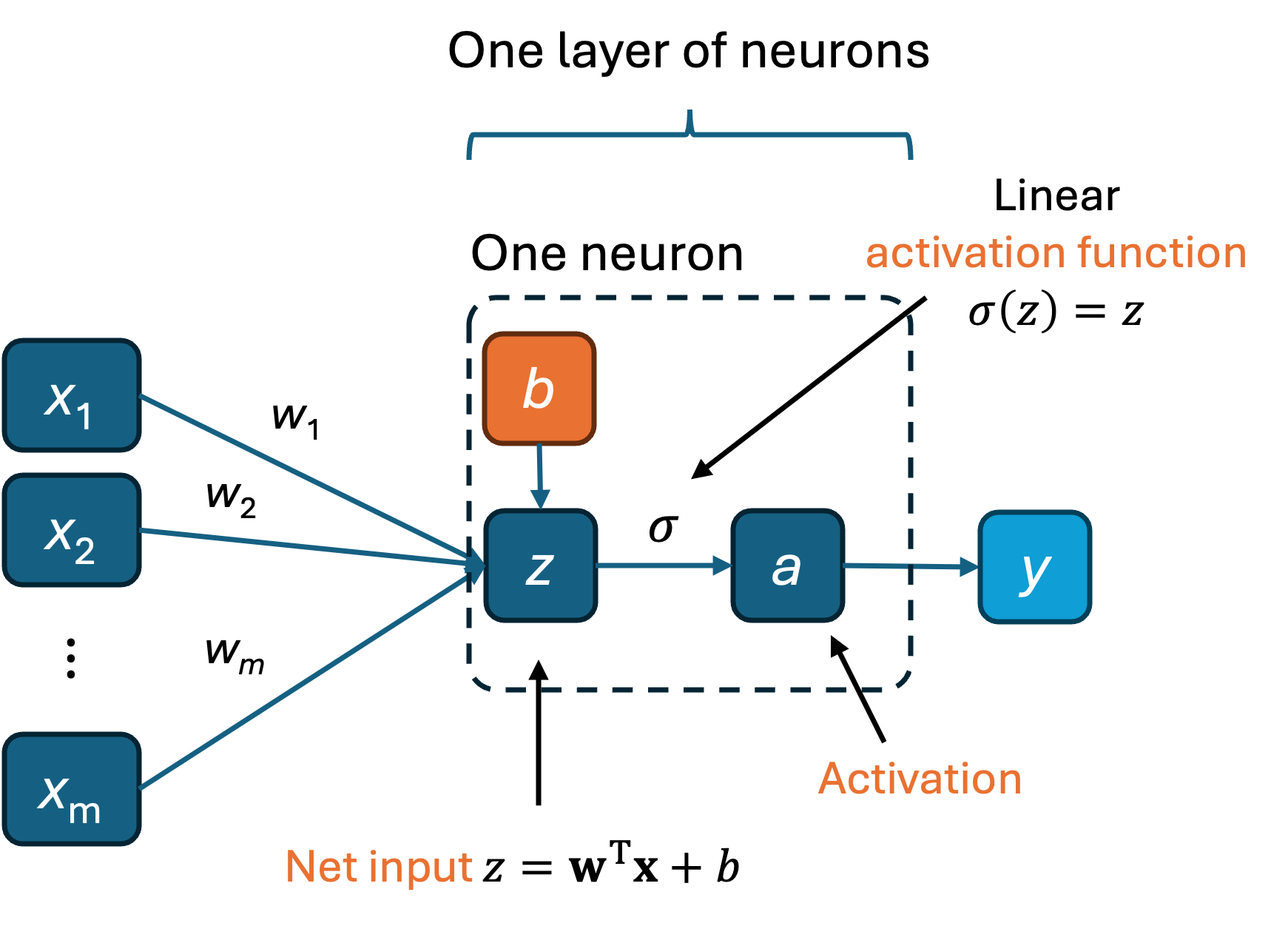
The same computation can be drawn as a one-neuron network in two steps:
- the net input is the weighted sum plus a bias (the intercept), \(z = \mathbf{w}^\top \mathbf{x} + b\);
- the activation applies an activation function \(\sigma\) to the net input, \(a = \sigma(z)\).
For linear regression the activation function is the identity, \(\sigma(z) = z\), and the activation \(a\) is taken as the prediction \(y\). The formulation is mathematically identical to linear regression; only the presentation is new. A neural network is obtained from this starting point by adding more neurons, and crucially non-linear activation functions.
8.2 Anatomy of a Neural Network
A feed-forward network arranges neurons into layers:
- the input layer holds the feature vector \(\mathbf{x}\);
- one or more hidden layers transform the data; and
- the output layer produces the prediction. For a single-target regression it contains one neuron, which recovers linear regression when there are no hidden layers.
Each layer performs the same two operations introduced above, now in vector form. For a layer with weight matrix \(\mathbf{W}\) and bias \(\mathbf{b}\),
\[ \mathbf{z} = \mathbf{x}\,\mathbf{W}^\top + \mathbf{b}, \qquad \mathbf{a} = \sigma(\mathbf{z}). \]
The activations of the output layer are the model’s predictions.
The standard architecture is the multi-layer perceptron (MLP), also called a feed-forward neural network. Its layers are fully connected: every neuron in a layer receives input from every neuron in the previous layer, so each connection carries its own weight. Two neurons within the same layer share the same functional form and differ only in their weights and bias, which are the parameters learned during training.
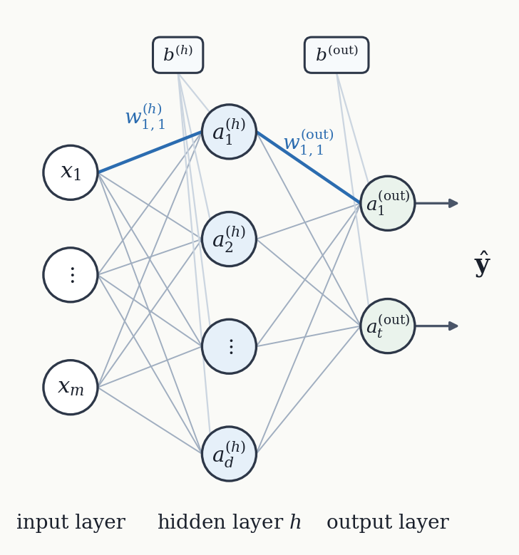
Computation proceeds layer by layer, with the activations of one layer serving as the input to the next. For a hidden layer, starting from the input \(\mathbf{x}^{(\text{in})}\),
\[ \mathbf{z}^{(h)} = \mathbf{x}^{(\text{in})}\,\mathbf{W}^{(h)\top} + \mathbf{b}^{(h)}, \qquad \mathbf{a}^{(h)} = \sigma\!\left(\mathbf{z}^{(h)}\right), \]
and for the output layer,
\[ \mathbf{z}^{(\text{out})} = \mathbf{a}^{(h)}\,\mathbf{W}^{(\text{out})\top} + \mathbf{b}^{(\text{out})}, \qquad \mathbf{a}^{(\text{out})} = \sigma\!\left(\mathbf{z}^{(\text{out})}\right). \]
Stacking \(n\) data points as rows of a matrix \(\mathbf{X}\) allows an entire batch to be processed in a single matrix multiplication, which is far more efficient than looping over points. This forward sweep of calculations, from inputs to predictions, is the forward pass.
8.3 Activation Functions
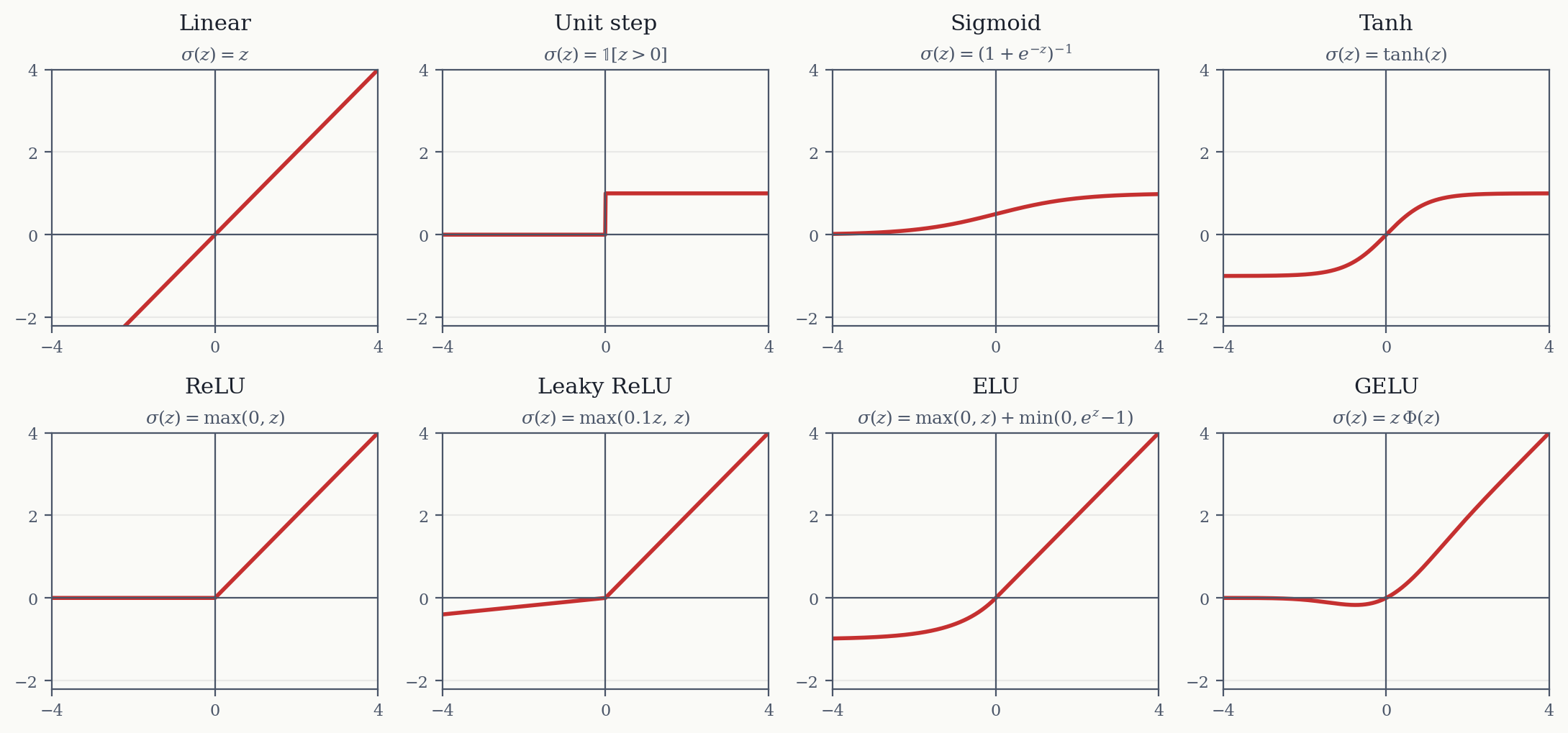
Without non-linear activation functions a multi-layer network would collapse into a single linear map, since a composition of linear functions is itself linear. The activation function is therefore what gives the network its expressive power, and its choice is an additional hyperparameter.
Early networks used the sigmoid and tanh functions, inspired by the saturating response of biological neurons. But this behaviour can cause problems with the training process since their gradient is close to zero for large positive or negative inputs, so numerous alternatives have been developed.
8.4 Training a Neural Network
Training a neural network uses the same principle as training linear regression: the weights are adjusted by gradient descent to minimize a loss function. The new ingredient is backpropagation, an efficient method for computing the gradient of the loss with respect to every weight in the network.
8.4.1 The loss function
For regression the standard loss is the mean squared error,
\[ \mathcal{L}(\mathbf{W}, \mathbf{b}) = \frac{1}{n}\sum_{i=1}^{n}\left(y^{(i)} - \hat{y}^{(i)}\right)^2, \]
where \(\hat{y}^{(i)}\) is the network’s output for point \(i\). The weights are then updated in the direction that decreases the loss, scaled by the learning rate \(\eta\):
\[ \mathbf{W}^{\text{next}} = \mathbf{W}^{\text{current}} - \eta\, \nabla_{\mathbf{W}}\mathcal{L}(\mathbf{W}, \mathbf{b}). \]
The only difficulty is computing the gradient \(\nabla_{\mathbf{W}}\mathcal{L}\) for a network with many layers.
8.4.2 Backpropagation
The forward pass shows how to compute the output from the inputs and weights. Backpropagation runs this dependency in reverse, applying the chain rule to propagate the loss back to every weight.
Consider a weight \(w^{(\text{out})}_{1,1}\) in the output layer. The required derivative factorizes into three terms:
\[ \frac{\partial \mathcal{L}}{\partial w^{(\text{out})}_{1,1}} = \frac{\partial \mathcal{L}}{\partial a^{(\text{out})}_{1}} \cdot \frac{\partial a^{(\text{out})}_{1}}{\partial z^{(\text{out})}_{1}} \cdot \frac{\partial z^{(\text{out})}_{1}}{\partial w^{(\text{out})}_{1,1}}. \]
Each factor is known from the forward pass:
- the derivative of the loss with respect to the last activation, for the squared error, is \(\dfrac{\partial \mathcal{L}}{\partial a^{(\text{out})}_{1}} = 2\left(a^{(\text{out})}_{1} - y_1\right)\);
- the derivative of the activation with respect to the net input is \(\sigma'(z^{(\text{out})}_1)\), which for the sigmoid equals \(a^{(\text{out})}_1\big(1 - a^{(\text{out})}_1\big)\);
- the derivative of the net input with respect to the weight is simply the upstream activation, \(\dfrac{\partial z^{(\text{out})}_{1}}{\partial w^{(\text{out})}_{1,1}} = a^{(h)}_1\).
The gradients for the hidden layers follow the same pattern, with one additional chain-rule factor per layer that the loss must pass through. Because every factor reuses quantities already computed during the forward pass, the full gradient is obtained in a single backward sweep, which is what makes training large networks feasible.
8.4.3 Flavors of gradient descent
The weight update can use different amounts of data per step:
- Batch (full) gradient descent uses the entire training set for every update. One pass over all the data is one epoch. Training a network requires many epochs.
- Stochastic gradient descent (SGD) uses a single randomly chosen data point per step. The updates are noisy but cheap.
- Mini-batch gradient descent uses a small random subset (for example 32 points) per step. This is the standard choice for neural networks, balancing the stability of batch descent against the efficiency of SGD.
The choice is largely driven by computational considerations, such as how efficiently the hardware can process a given batch size.
8.5 Regularization
Neural networks have many parameters and can overfit readily, so regularization is essential. The methods fall into two groups.
Explicit regularization adds a penalty to the loss or constrains the weights directly:
- L2 (ridge) weight penalty, in this context usually called weight decay;
- L1 (lasso) weight penalty, which encourages sparse weights;
- max-norm regularization, which caps the magnitude of each weight vector.
Implicit regularization constrains the model without an explicit penalty term, and is the more common choice in practice:
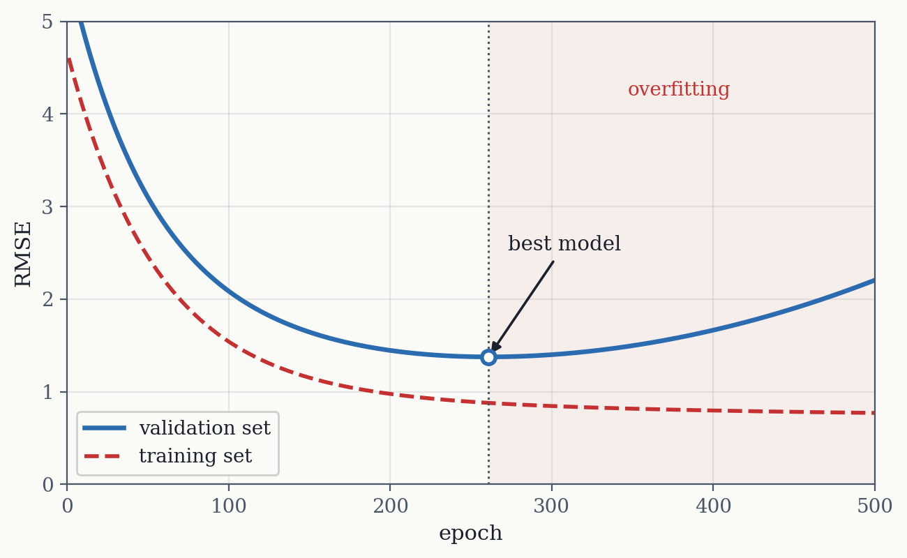
- Early stopping halts training when the validation error stops decreasing, returning the weights at the validation minimum (see Figure 8.1 below).
- Dropout randomly ignores a fraction of neurons (typically 10–50%) at each training step. This forces the network to spread its representation across many connections rather than relying on a few, and is equivalent to averaging over an ensemble of subnetworks. At evaluation time all neurons are used.
8.6 Some Practical Notes
- Neural networks expose many hyperparameters concerning both their architecture and optimization and tuning them can be very expensive, which makes regularization even more important.
- For tabular chemical data, gradient boosting and kernel methods are usually preferable. Feed-forward networks on tabular data tend to require disproportionate tuning effort relative to their benefit, as noted in the previous chapter.
- The principal value of neural networks is as a building block. Stacking and specializing the layers introduced here yields the graph neural networks and language models that are the subject of the following chapters.
- Neural networks perform representation learning: earlier layers learn general building blocks and later layers combine them into task-specific patterns, a property that becomes central in those later models.
8.7 Summary
- From neuron to network. A neuron computes a net input \(z = \mathbf{w}^\top\mathbf{x} + b\) followed by an activation \(a = \sigma(z)\). With the identity activation this is exactly linear regression; a network is obtained by adding more neurons and, crucially, non-linear activations.
- Architecture. The multi-layer perceptron stacks fully connected layers — input, one or more hidden, output — each applying \(\mathbf{z} = \mathbf{x}\mathbf{W}^\top + \mathbf{b}\), \(\mathbf{a} = \sigma(\mathbf{z})\). Stacking data points into a matrix lets a whole batch be processed in one matrix multiplication. This sweep from inputs to predictions is the forward pass.
- Activation functions supply the expressive power: without them a deep network collapses to a single linear map. Sigmoid and tanh saturate, giving near-zero gradients for large inputs, which motivated the many alternatives now in use.
- Training minimizes the loss by gradient descent, with backpropagation computing every weight’s gradient in a single backward sweep by applying the chain rule and reusing quantities from the forward pass. This is what makes large networks trainable at all.
- Flavors of gradient descent differ in how much data each update uses: batch (all data, one pass = one epoch), stochastic (one point, cheap and noisy), and mini-batch (typically tens to hundreds of points), which is the standard choice.
- The loss landscape is non-convex, unlike linear regression, so there is no guarantee of finding the global minimum — but many local minima perform comparably, and the noise in mini-batch updates helps escape poor ones. Ill-conditioned (elongated) loss surfaces can hinder optimization, and too large a learning rate can cause divergence.
- Regularization is essential given the parameter count. Explicit: L2 (weight decay), L1, max-norm. Implicit and more commonly used: early stopping at the validation minimum, and dropout, which randomly disables 10–50% of neurons per step, effectively averaging over an ensemble of subnetworks.
- In practice, feed-forward networks are rarely the best choice for tabular chemical data — gradient boosting and kernel methods usually win for less tuning effort. Their real value is as a building block: the layers introduced here, specialized and stacked, become the graph and language models of the following chapters, and their representation learning behaviour is what those models exploit.