10 Language Models
The graph models chapter treated molecules as graphs and let a neural network learn a representation directly from atoms and bonds. This chapter develops the second major representation-learning approach for chemistry: treating a molecule as a sequence, in the same way that a sentence is a sequence of words. A convenient sequential encoding of a molecule is its SMILES string, and the models that operate on such sequences are language models.
Both approaches share the philosophy introduced for neural networks: rather than feeding a model fixed expert descriptors, the input is given in a raw structured form and the network learns the representation best suited to the task. Where graph models read the molecular graph, language models read the character sequence.
We will start with Recurrent neural networks (RNNs) as a simple model architecture for sequential data and introduce the core ideas. Their limitations motivate the attention mechanism, which in turn leads to the transformer, the architecture underlying essentially every modern language model. The chapter closes with more recent developments of that architecture for chemistry: foundation models, transfer learning, and LLM agents.
10.1 Molecules as Sequences
10.1.1 Sequential data
The data encountered so far in this course has had no intrinsic ordering. The bits of a fingerprint, for instance, can be permuted without changing the molecule they describe; their position carries no special meaning. Sequential data is different: the order of the elements is part of the information, because later elements are related to earlier ones. Time series, audio, and natural language are all sequential, and so are SMILES strings. Reordering the tokens of a sequence changes its meaning, which is why sequential data requires its own family of models – classical methods such as ARIMA for time series, and recurrent or attention-based neural networks for deep learning.
10.1.2 SMILES tokens and the vocabulary
To process a SMILES string a model first splits it into tokens, the atomic units of the sequence. The complete set of defined tokens is the vocabulary. A natural tokenization keeps each chemically meaningful unit as one token:
SMILES:     ClC1=CC(C)=CC(C)=C1
tokenized:  Cl  C  1  =  C  C  (  C  )  =  C  C  (  C  )  =  C  1
Note that the two-letter element symbol Cl is kept as a single token rather than being split into C and l. This is one possible scheme; as in natural-language processing, one could also tokenize at the level of characters or of recurring sub-words. The choice of tokenization is a design decision that affects vocabulary size and model behaviour.
10.1.3 What we want to do with sequences
Two broad tasks recur throughout the chapter:
- Property prediction, mapping an input sequence to a scalar (or a class). For example, the SMILES of a molecule is mapped to its solubility.
- Generation and translation, mapping an input sequence to an output sequence. Forward reaction prediction, for example, maps the SMILES of the reactants to the SMILES of the products.
The same underlying machinery – learn a representation of the sequence, then read a prediction off that representation – serves both.
10.2 Recurrent Neural Networks
10.2.1 The recurrent neuron
A standard feed-forward network maps a fixed-size input vector to an output in a single pass. To handle a sequence it is modified by introducing recurrence. A recurrent neuron processes the sequence one token at a time and, crucially, receives at each step not only the current input but also its own output from the previous step. This recycled quantity is the hidden state, and it acts as a memory that lets earlier tokens influence the processing of later ones.
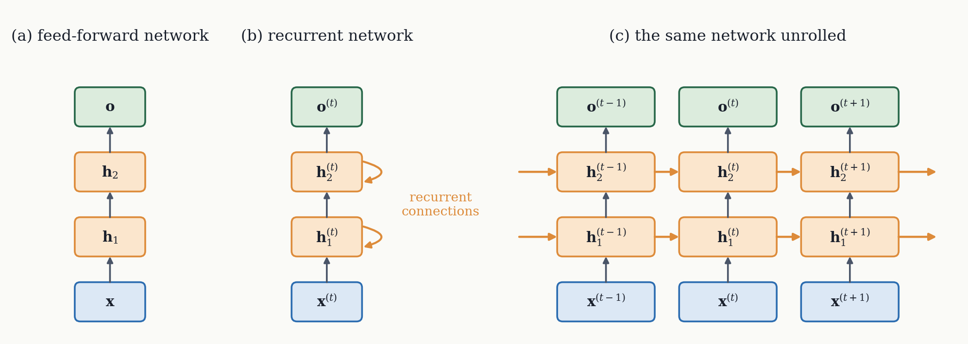
The compact recurrent diagram, with its self-loop, is most easily read after unrolling it in time: the loop is written out as one copy of the neuron per position in the sequence, the copies connected left to right. Each copy processes its token, passes its hidden state to the next, and optionally emits an output.
10.2.2 The mathematics of an RNN
At sequence position \(t\), with input token (embedding) \(\mathbf{x}^{(t)}\) and previous hidden state \(\mathbf{h}^{(t-1)}\), the recurrent layer computes a net input
\[ \mathbf{z}_h^{(t)} = \mathbf{W}_{xh}\,\mathbf{x}^{(t)} + \mathbf{W}_{hh}\,\mathbf{h}^{(t-1)} + \mathbf{b}_h, \]
a hidden state
\[ \mathbf{h}^{(t)} = \sigma_h\!\left(\mathbf{z}_h^{(t)}\right), \]
and an output
\[ \mathbf{o}^{(t)} = \sigma_o\!\left(\mathbf{W}_{ho}\,\mathbf{h}^{(t)} + \mathbf{b}_o\right). \]
The term \(\mathbf{W}_{hh}\,\mathbf{h}^{(t-1)}\), absent from an ordinary feed-forward layer, is what makes the network recurrent. At the first position there is no previous state, so \(\mathbf{h}^{(0)} = \mathbf{0}\). The weight matrices \(\mathbf{W}_{xh}\), \(\mathbf{W}_{hh}\), and \(\mathbf{W}_{ho}\) are shared across all time steps: the same neuron, with the same parameters, is applied at every position. As with feed-forward networks, recurrent layers can be stacked, each layer receiving at every step both its own previous hidden state and the current hidden state of the layer below.
10.2.3 From tokens to input vectors: the embedding layer
The recurrent equations require a continuous vector \(\mathbf{x}^{(t)}\) for each token, but a token is initially just a symbol. The conversion is performed by an embedding layer. Each token is first one-hot encoded against the vocabulary, then passed through a linear layer whose weights map the sparse one-hot vector to a dense, continuous embedding. These embedding weights are learned during training together with the rest of the network. A well-known side effect is that the learned embeddings become meaningful: tokens that play similar roles end up close together in the embedding space.
10.3 Output Configurations
What an RNN produces depends on which outputs are read. Three configurations cover the common cases.
- Sequence-to-vector (many-to-one). The whole input sequence is processed and only the final output is used. This is the setup for property prediction: the SMILES is fed in token by token, and the output after the last token is passed to a regression or classification head to predict, say, solubility or toxicity. A useful trick here is SMILES augmentation (enumeration): because a molecule has many valid non-canonical SMILES, generating several of them multiplies the training data and helps the model learn the syntax of SMILES.
- Vector-to-sequence (one-to-many). A single input is expanded into a sequence, as in image captioning or molecular generation.
- Sequence-to-sequence (many-to-many). An input sequence is mapped to an output sequence, as in translation or reaction prediction. The encoder–decoder architecture is the usual choice for this type of task.
10.3.1 The encoder–decoder for reaction prediction
In forward reaction prediction the reactant SMILES is mapped to the product SMILES. An encoder RNN first consumes the reactant sequence token by token; its intermediate outputs are discarded, but its final hidden state – a summary of the entire input – is passed to a decoder RNN. The decoder is started with a special token and generates the product one token at a time. Each generated token is fed back in as the input for the next step, a procedure called autoregression, and generation continues until the model emits a special end-of-sequence token.
10.3.2 Generating tokens: softmax, temperature, and sampling
At each decoding step the model must choose the next token. Its final layer produces one score per vocabulary entry, and these are turned into probabilities by the softmax function, the multi-class generalization of the logistic sigmoid \(\sigma(z) = 1/(1 + e^{-z})\) used in binary classification:
\[ p(z_i) = \frac{e^{\,z_i / T}}{\sum_{j=1}^{K} e^{\,z_j / T}}. \]
Given the probabilities, the next token can be chosen in two ways. Greedy decoding always takes the most probable token; this is safe but repetitive. Sampling instead draws a token at random according to the probabilities, which produces more varied output. The parameter \(T\) is the temperature, which rescales the scores before the softmax:
- low temperature sharpens the distribution toward the highest-scoring tokens, giving precise, conservative output;
- high temperature flattens the distribution toward uniform, giving more diverse, “creative” output.
This is the same temperature setting exposed by many chatbots. More elaborate strategies such as top-\(k\) sampling and beam search also exist. The widget shows how temperature reshapes the distribution over a small SMILES vocabulary.
#| '!! shinylive warning !!': |
#|   shinylive does not work in self-contained HTML documents.
#|   Please set `embed-resources: false` in your metadata.
#| standalone: true
#| viewerHeight: 540

from shiny import App, render, ui
import numpy as np
import matplotlib.pyplot as plt
import matplotlib

matplotlib.rcParams.update({
    "font.family": "serif",
    "figure.facecolor": "#fafaf7",
    "axes.facecolor": "#fafaf7",
    "axes.grid": True,
    "grid.alpha": 0.3,
})

BLUE = "#2b6cb0"
RED = "#c53030"
ORANGE = "#e8833a"
GREEN = "#276749"
PURPLE = "#805ad5"

# Fixed model scores (logits) over a small next-token vocabulary
TOKENS = ["C", "c", "(", ")", "=", "O", "N", "1", "<eos>"]
LOGITS = np.array([3.0, 1.6, 0.8, 0.4, 1.3, 2.1, 0.5, 1.0, -0.3])

app_ui = ui.page_fluid(
    ui.input_slider("temp", "Temperature T", min=0.1, max=3.0,
                    value=1.0, step=0.05),
    ui.output_plot("softmax_plot"),
)


def server(input, output, session):
    @render.plot
    def softmax_plot():
        T = input.temp()
        z = LOGITS / T
        z = z - z.max()
        p = np.exp(z)
        p = p / p.sum()

        greedy = int(np.argmax(p))
        colors = [ORANGE if i == greedy else BLUE for i in range(len(TOKENS))]

        fig, ax = plt.subplots(figsize=(6, 4))
        ax.bar(np.arange(len(TOKENS)), p, color=colors, edgecolor="#333", linewidth=0.6)
        ax.set_xticks(np.arange(len(TOKENS)))
        ax.set_xticklabels(TOKENS)
        ax.set_ylim(0, 1.0)
        ax.set_ylabel("probability")
        ax.set_xlabel("next token")
        fig.tight_layout()
        return fig


app = App(app_ui, server)
At \(T \to 0\) the distribution collapses onto the single most probable token, recovering greedy decoding; at large \(T\) the tokens become nearly equiprobable and sampling produces highly varied, often invalid, SMILES.
10.4 The Attention Mechanism
The encoder–decoder RNN has a structural bottleneck: all information about the input must pass through a single fixed-size hidden state handed from encoder to decoder. The model therefore struggles to “remember” tokens that occurred early in a long input. This matters for chemistry, because atoms that interact in a reaction can be far apart in the SMILES string, and a plain RNN tends to mishandle such long-range dependencies.
The attention mechanism removes the bottleneck by giving the decoder direct access to every encoder state. At each decoding step \(t\) the decoder receives, in addition to its own hidden state, a context vector formed as a weighted average of all the encoder outputs \(\hat{\mathbf{y}}^{(i)}\):
\[ \mathbf{c}_t = \sum_{i} \alpha_{t,i}\,\hat{\mathbf{y}}^{(i)}. \]
The attention weights \(\alpha_{t,i}\) are computed dynamically by a small auxiliary network, the alignment model, from the decoder’s current state and each encoder output; the resulting alignment scores are normalized with a softmax so that they sum to one. Because the weights are recomputed at every decoding step, the decoder can focus on different parts of the input at different times, and – decisively – it can attend to a relevant token regardless of how far away that token sits in the sequence. Attention substantially eases the memory problem of RNNs, but the recurrence itself remains a bottleneck for training, which motivates discarding it entirely.
10.5 The Transformer
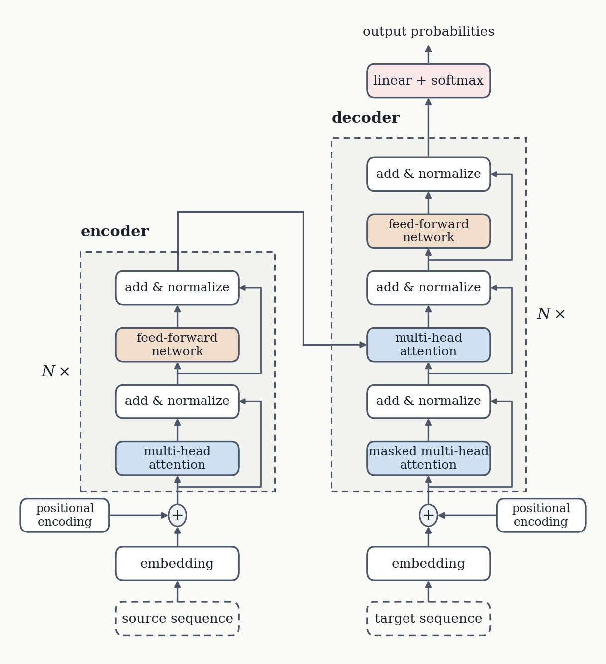
The transformer takes the lesson of attention to its conclusion: attention is all you need. The recurrent connections are removed altogether, and attention becomes the only mechanism for moving information between positions. The encoder–decoder structure is retained – the encoder builds a contextualized representation of the input, and the decoder generates the output autoregressively – but every recurrent neuron is replaced by attention layers. The Figure below shows a conceptual visualisation of the architecture and we will now go through its most important building blocks.
10.5.1 Self-attention
The core operation is self-attention, in which each token is re-embedded using information from all the tokens in the same sequence (including itself). In its simplest form, the contribution of token \(j\) to the new embedding of token \(i\) is governed by their similarity, measured as a dot product. You can see the relevant equations below. The dot products are normalized with a softmax to give attention weights, and the new embedding is the weighted average of the token vectors. The result is a context-aware embedding: a single vector for one token that nevertheless carries information from the whole sequence.
10.5.2 Key, query, and value
The parameterized version used in practice borrows terminology from information retrieval. For each input token three vectors are produced by three learned matrices \(\mathbf{U}_q\), \(\mathbf{U}_k\), \(\mathbf{U}_v\):
- the query \(\mathbf{q}^{(i)}\) – what the current token is “looking for”;
- the key \(\mathbf{k}^{(i)}\) – what each token “offers”, matched against queries;
- the value \(\mathbf{v}^{(i)}\) – the content actually aggregated.
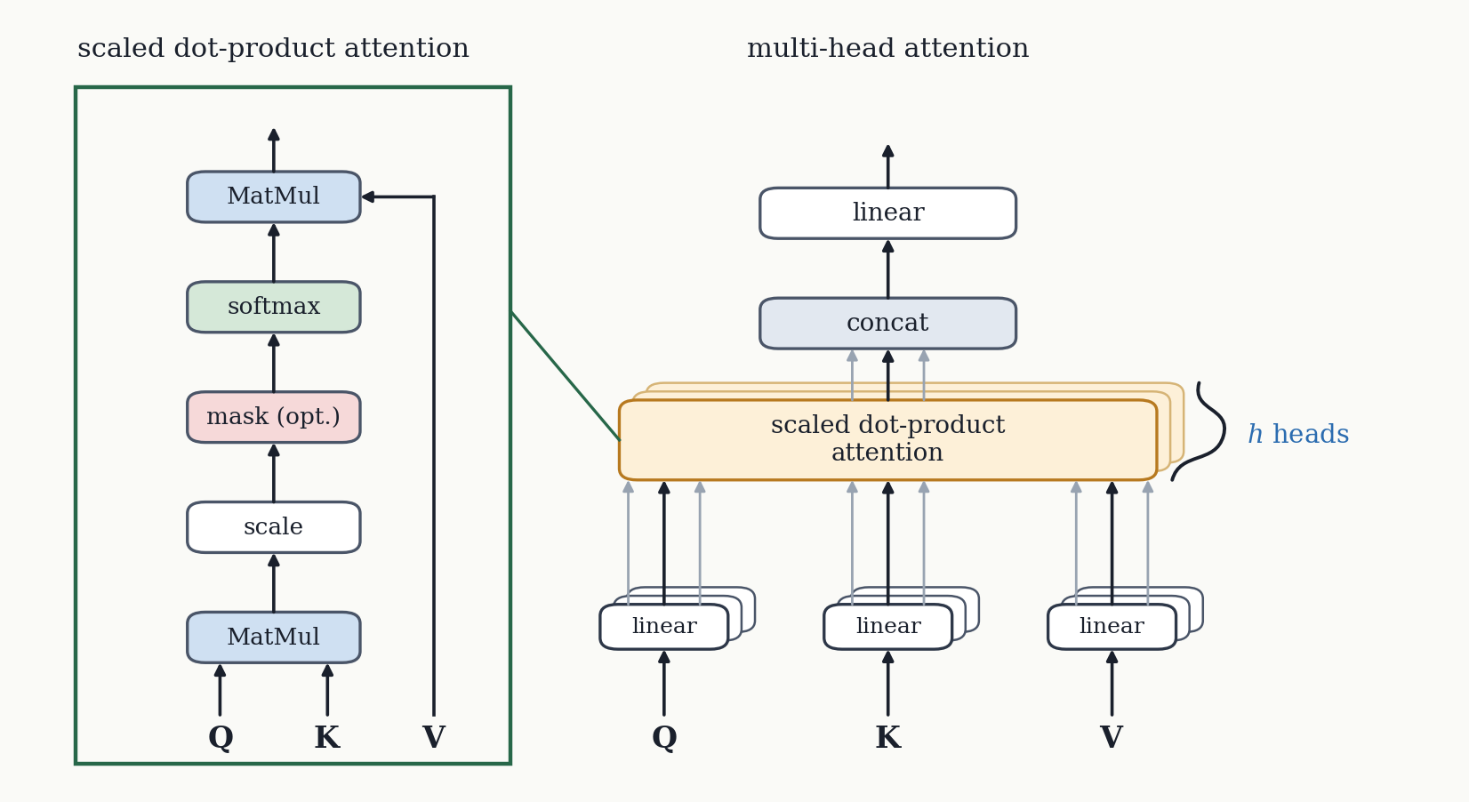
A query is compared against all keys to obtain unnormalized weights, which are normalized and then used to weight the values. In scaled dot-product self-attention the scores are divided by the square root of the embedding dimension \(d\) to keep them in a stable range:
\[ \omega_{i,j} = \mathbf{q}^{(i)\top}\mathbf{k}^{(j)}, \qquad \alpha_{i,j} = \mathrm{softmax}\!\left(\frac{\omega_{i,j}}{\sqrt{d}}\right), \qquad \mathbf{z}^{(i)} = \sum_{j} \alpha_{i,j}\,\mathbf{v}^{(j)}. \]
Because the matrices \(\mathbf{U}_q\), \(\mathbf{U}_k\), \(\mathbf{U}_v\) are learned, this version is far more flexible than the parameter-free dot-product form.
10.5.3 Multi-head attention
A single attention layer captures one notion of relevance. Multi-head attention runs several attention layers, or heads, in parallel, each with its own set of query, key, and value matrices. Each head can therefore focus on a different aspect of the sequence. The per-head output embeddings are concatenated and passed through a linear layer that restores the original dimensionality.
10.5.4 Attention in the decoder
The decoder uses two specialized forms of attention. Masked self-attention prevents the model, during training, from attending to tokens it has not yet generated: future positions are hidden (“masked”) so the model cannot cheat by looking ahead. This causal masking is exactly why a decoder’s attention matrix is lower-triangular – each position may attend only to itself and to earlier positions. Cross-attention then mixes the decoder’s representation with the encoder’s output, the transformer’s analogue of passing information from input to output. Several further components – positional encodings (which inject token order, lost when recurrence is removed), skip connections, and normalization layers – complete the architecture; they are important in practice but are not detailed here.
10.5.5 Interactive example: self-attention
The widget computes self-attention over the tokenized SMILES of acetic acid, C C ( = O ) O. Each token is given a small fixed embedding in which chemically similar tokens (the two carbons; the two oxygens; the matching brackets) point in similar directions. The heatmap shows the attention weight from each query token (row) to each key token (column). Two options reproduce features of the transformer: scaling the scores by \(\sqrt{d}\), and applying the causal mask used in the decoder.
#| '!! shinylive warning !!': |
#|   shinylive does not work in self-contained HTML documents.
#|   Please set `embed-resources: false` in your metadata.
#| standalone: true
#| viewerHeight: 600

from shiny import App, render, ui
import numpy as np
import matplotlib.pyplot as plt
import matplotlib

matplotlib.rcParams.update({
    "font.family": "serif",
    "figure.facecolor": "#fafaf7",
    "axes.facecolor": "#fafaf7",
})

# Tokenized SMILES of acetic acid
TOKENS = ["C", "C", "(", "=", "O", ")", "O"]
TYPE = {"C": 0, "(": 1, "=": 2, "O": 3, ")": 1}  # ')' resembles '('
D = 8

# Build fixed, interpretable embeddings: a base vector per token type + small noise
rng = np.random.default_rng(1)
type_vecs = rng.normal(size=(4, D))
E = np.array([type_vecs[TYPE[t]] for t in TOKENS]) + rng.normal(scale=0.25, size=(len(TOKENS), D))
E = E / np.linalg.norm(E, axis=1, keepdims=True)


def softmax_rows(x):
    x = x - np.max(x, axis=1, keepdims=True)
    e = np.exp(x)
    return e / np.sum(e, axis=1, keepdims=True)


app_ui = ui.page_fluid(
    ui.layout_columns(
        ui.input_checkbox("scaled", "Scale scores by sqrt(d)", value=True),
        ui.input_checkbox("mask", "Causal mask (decoder)", value=False),
    ),
    ui.output_plot("attn_plot"),
)


def server(input, output, session):
    @render.plot
    def attn_plot():
        omega = E @ E.T
        if input.scaled():
            omega = omega / np.sqrt(D)
        if input.mask():
            n = len(TOKENS)
            causal = np.triu(np.ones((n, n), dtype=bool), k=1)  # future positions
            omega = np.where(causal, -np.inf, omega)
        alpha = softmax_rows(omega)

        fig, ax = plt.subplots(figsize=(6, 5))
        im = ax.imshow(alpha, cmap="Reds", vmin=0.0, vmax=1.0)
        ax.set_xticks(np.arange(len(TOKENS)))
        ax.set_yticks(np.arange(len(TOKENS)))
        ax.set_xticklabels(TOKENS)
        ax.set_yticklabels(TOKENS)
        ax.set_xlabel("key token (attended to)")
        ax.set_ylabel("query token")
        for i in range(len(TOKENS)):
            for j in range(len(TOKENS)):
                v = alpha[i, j]
                if v > 0.005:
                    ax.text(j, i, f"{v:.2f}", ha="center", va="center",
                            fontsize=8, color=("white" if v > 0.5 else "#333"))
        fig.colorbar(im, ax=ax, fraction=0.046, pad=0.04, label="attention weight")
        ax.set_title("Self-attention weights for  C C ( = O ) O", fontsize=11)
        fig.tight_layout()
        return fig


app = App(app_ui, server)
Each row sums to one: it is the distribution of attention that one query token places over the sequence. Like tokens attend to like tokens – the two carbons reinforce each other, as do the two oxygens. Disabling the \(\sqrt{d}\) scaling sharpens the weights; enabling the causal mask zeroes out the upper triangle, leaving the lower-triangular pattern characteristic of decoder self-attention.
10.6 Transformers in Chemistry
The transformer has rapidly become the dominant architecture in both general machine learning and chemistry. The molecular transformer is one example where Philippe Schwaller and co-workers introduced the transformer architecture for reaction prediction and achieved markedly better performance than previous RNN models, especially for larger molecules whose SMILES contain the long-range dependencies that recurrence handles poorly.
Most transformer-based chemistry models derive from one of two reductions of the full encoder–decoder:
- Encoder-only models (BERT-type) keep only the encoder and use non-masked, bidirectional self-attention, so every token attends to the whole sequence. They are well suited to producing a representation of a complete input, for example for classification or property prediction.
- Decoder-only models (GPT-type) keep only the decoder and use masked, unidirectional attention. They are trained on next-token prediction and are the basis of generative language models.
In practice one rarely trains such models from scratch. The standard workflow is to download a chemistry-related model that has already been pre-trained – for example from the Hugging Face hub – and adapt it, using a library such as transformers.
10.7 Foundation Models
10.7.1 The idea
A neural network learns a representation of its input in its hidden layers; the activations of the last layer before the output, the latent space, are a learned vector representation of the input, as discussed for neural networks. The premise of a foundation model is that the principles underlying many tasks are shared. A single model is trained on a very large dataset to produce a general-purpose representation that reflects these shared principles, and that representation is then reused – or lightly adapted – for many downstream tasks through transfer learning.
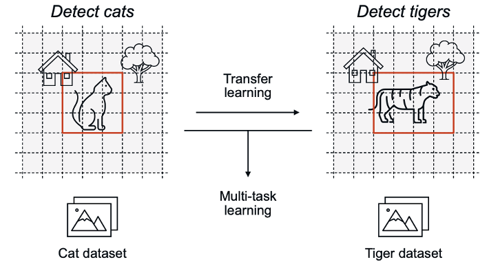
10.7.2 Adapting a foundation model
Two strategies adapt a pre-trained foundation model to a new task:
- Feature extraction (frozen base). The foundation model’s weights are kept frozen and used only to generate the latent representation. New output layers are trained on top of it. The head need not be a neural network – it can be any model, for example a kernel or a gradient-boosting regressor on the extracted features.
- Fine-tuning. All weights, including those of the foundation model, are updated on the new task, optionally after adding new layers. This is more powerful but requires more data and computation.
10.7.3 Self-supervised pre-training
Foundation models need enormous training sets, which are difficult to obtain when each label requires an experiment. Self-supervised learning sidesteps this by manufacturing training signal from unlabeled data through artificial tasks. Language models are pre-trained with next-word, next-sentence, and masked-token prediction: a token in the input is hidden and the model must reconstruct it. For SMILES this means masking an atom or bond in a string and asking the model to predict it,
O=C(O)c1ccccc1C(=O)O -> O=C(O)c1cc[MASK]cc1C(=O)O -> predict: cSolving such tasks forces the model to learn the syntax and regularities of SMILES, yielding a representation usable for many downstream property predictions.
10.7.4 Example: the RXNFP reaction fingerprint
A concrete example is RXNFP, a reaction fingerprint built from a BERT-type (encoder-only) transformer. The model is first pre-trained with masked-language modeling on reaction SMILES, then fine-tuned to predict reaction class. The learned representation is read from a special token ([CLS]) of the final layer, giving a fixed-length, context-aware vector for the whole reaction. Both the pre-trained and the fine-tuned versions are foundation models in the sense above, and the resulting fingerprints have been used as inputs to downstream models – combined with Gaussian process regression or feed-forward networks – to predict, for instance, reaction activation energies.
10.7.5 In-context learning
Large decoder-only models exhibit a further mode of adaptation that requires no weight updates at all: the task is described in natural language directly in the prompt, and the answer is produced in natural language. Depending on how many worked examples the prompt contains, this is called zero-shot, one-shot, or few-shot learning.
10.8 From Transformer to Chatbot and LLM Agents
A raw transformer trained on next-token prediction is a base model. Turning it into a usable chatbot requires further steps: fine-tuning on conversational data and on human feedback, followed by deployment with surrounding engineering. The most capable systems go beyond a bare model and become augmented LLMs equipped with tools and memory.
- Tools let the model delegate tasks it performs poorly. The model writes a structured request (for example a JSON call) to an external program; the program runs and its result is fed back into the model. A calculator tool, for instance, lets the model answer arithmetic reliably, which next-token prediction alone does not.
- Memory extends the model beyond a single response. Short-term memory simply appends the conversation history to the prompt and is bounded by the context length, which modern models have pushed to hundreds of thousands or even millions of tokens. Long-term memory persists across sessions; a common implementation is retrieval-augmented generation (RAG), in which documents are embedded into a vector database, the most similar passages to an embedded query are retrieved, and their text is injected into the prompt.
Model quality can also be improved at inference time by chain-of-thought reasoning, prompting the model to work through a problem in explicit steps rather than answering immediately.
An LLM agent combines these capabilities with planning: the model decides which actions to take, gathers information from tools, stores results in memory, and chooses subsequent steps until the task is complete. In chemistry, such agents – for example Coscientist and ChemCrow – couple a language model to chemistry tools and even to laboratory automation, using the model as a planner that calls specialized tools (some of which are themselves models or physical experiments) and integrates their results.
10.9 Summary
Language models provide an alternative to graph models for learning representations of molecules, operating on the sequential SMILES encoding rather than on the molecular graph. The chapter covered in order:
- Recurrent neural networks process sequences with a recurrent hidden state, trained by backpropagation through time, but their inner workings cause memory problems that limit the usable sequence length.
- Attention removes the memory bottleneck by letting the model draw on any part of the input directly, weighted by learned relevance.
- The transformer discards recurrence entirely and relies on self-attention, multi-head attention, and – in the decoder – masked and cross-attention. It is the architecture behind modern language models, and in chemistry behind tools such as the molecular transformer, BERT-type encoders, and GPT-type decoders.
- Foundation models exploit the learned latent space: pre-trained on large datasets through self-supervised tasks, they are reused or fine-tuned for many downstream problems via transfer learning. LLM agents extend a language model with tools, memory, and planning.