7 Non-Linear Models
The chapter on linear models introduced models that express the target as a weighted sum of the input features, \(\hat{y} = \mathbf{w}^\top \mathbf{x}\). Such models are fast, interpretable, and often competitive, but they are restricted to linear decision boundaries and flat regression surfaces. Many problems in chemistry violate this assumption: a reaction may proceed only within a narrow window of temperature and concentration, a solubility may depend on a descriptor in a strongly curved manner, and classes are rarely separable by a single hyperplane.
This chapter introduces the principal families of non-linear supervised models used for tabular chemical data:
- Polynomial regression – a linear model fitted to an enriched set of higher-degree and cross terms.
- Tree-based methods – decision trees and the ensembles built from them: random forests (bagging) and gradient boosting (boosting).
- Kernel methods – linear models evaluated in an implicitly enlarged feature space, with kernel ridge regression as the principal example.
- Neural networks, which also fall in this category, will be treated in the following chapter.
A further kernel method, Gaussian process regression, is covered later in the context of Bayesian optimization.
7.1 Going Beyond Linearity
When a problem is not linearly solvable – the two classes cannot be divided by a single plane, or the regression trend is curved – the most direct remedy is to retain the linear formulation but enrich the feature set with higher-degree and cross terms:
\[ y = w_1 x_1 + w_2 x_2 + \underbrace{w_3 x_1^2 + w_4 x_2^2}_{\text{2nd-degree terms}} + \underbrace{w_5 x_1 x_2}_{\text{cross term}} + \cdots \]
This is polynomial regression: the features are mapped into a larger space, an ordinary linear model is fitted there, and the result corresponds to a curved fit in the original space.
However, this approach is limited due to computational effort and can overfit easily with high polynomial degrees \(d\) since the number of polynomial terms of degree \(d\) for \(m\) features grows factorially:
\[ \frac{(m + d)!}{d!\, m!}. \]
Explicitly constructing this enlarged feature space rapidly becomes infeasible for more than a handful of features or a modest degree and overfitting has to be controlled by regularization. Polynomial regression is thus a “brute-force” route to non-linearity, paid for with a rapidly growing feature space. The remaining models in this chapter reach non-linearity without an explicit expansion: decision trees partition the input space directly, tree ensembles combine many such partitions, and kernel methods operate in a non-linear space without ever constructing it explicitly.
7.2 Decision Trees
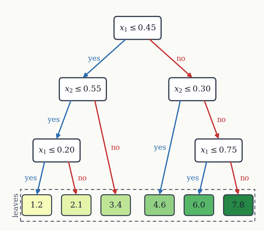
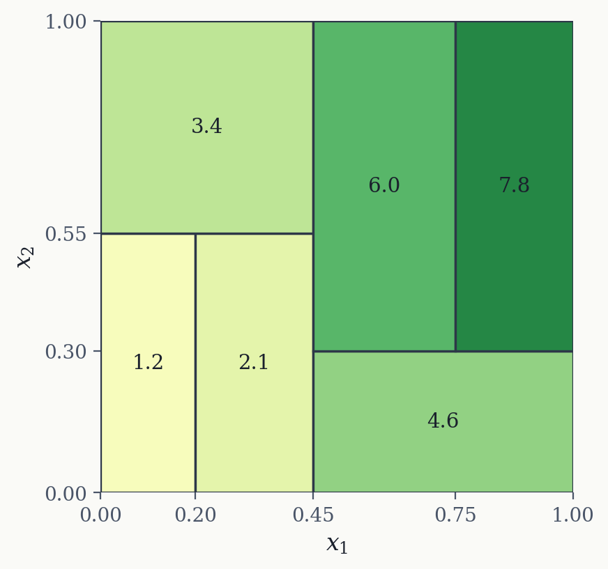
A decision tree predicts by asking a sequence of simple yes/no questions about the features. All samples enter at the root node, are routed through split nodes – each testing whether one feature lies above or below a threshold – and arrive at a leaf node that supplies the prediction. For regression the leaf returns the average of the training targets that reach it; for classification it returns the majority class. The resulting regression surface is therefore piecewise constant: the input space is carved into axis-aligned rectangles, each assigned a single value (Figure 7.1).
7.2.1 Training a tree: the CART algorithm
The standard training procedure is the Classification and Regression Tree (CART) algorithm. It is greedy and binary: at each node it searches over every feature \(k\) and threshold \(t_k\) for the single split that minimizes the combined loss of the two resulting children, weighted by the number of samples in each,
\[ \mathcal{L}(k, t_k) = \frac{n_\text{left}}{n_\text{parent}}\, \mathcal{L}_\text{left} + \frac{n_\text{right}}{n_\text{parent}}\, \mathcal{L}_\text{right}. \]
“Greedy” means each split is chosen to be locally optimal, with no regard for splits further down the tree. The node-level loss \(\mathcal{L}\) measures impurity. For regression it is the mean squared error about the node mean \(\hat{y}_i\),
\[ \text{MSE}_i = \frac{1}{n_i} \sum_{k=1}^{n_i} \left(\hat{y}_i - y_k\right)^2, \qquad \hat{y}_i = \frac{1}{n_i}\sum_{k=1}^{n_i} y_k. \]
For classification the default is the Gini impurity:
\[ G_i = 1 - \sum_{k} p_{i,k}^2, \]
where \(p_{i,k}\) is the fraction of class \(k\) among the samples at node \(i\). A pure node (one class only) has \(G_i = 0\). For example, a node holding 20 samples of class 0 and 40 of class 1 has
\[ G = 1 - \left(\left(\tfrac{20}{60}\right)^2 + \left(\tfrac{40}{60}\right)^2\right) = 0.44, \]
whereas a node containing only class 0 has \(G = 0\) and is not split further.
7.2.2 Overfitting and stopping criteria
Left unconstrained, a tree keeps splitting until every leaf is pure, memorizing the training data – decision trees have low bias but high variance and overfit readily. Growth is therefore limited by hyperparameters, the most important being the maximum depth. Others available in scikit-learn include min_samples_split, min_samples_leaf, min_weight_fraction_leaf, and max_leaf_nodes.
#| '!! shinylive warning !!': |
#|   shinylive does not work in self-contained HTML documents.
#|   Please set `embed-resources: false` in your metadata.
#| standalone: true
#| viewerHeight: 600

from shiny import App, render, ui
import numpy as np
import matplotlib.pyplot as plt
import matplotlib

matplotlib.rcParams.update({
    "font.family": "serif",
    "figure.facecolor": "#fafaf7",
    "axes.facecolor": "#fafaf7",
    "axes.grid": True,
    "grid.alpha": 0.3,
})

BLUE = "#2b6cb0"
RED = "#c53030"
GREEN = "#276749"

np.random.seed(11)
n = 80
x_data = np.linspace(-3, 3, n)
y_true = np.sin(1.2 * x_data) + 0.3 * x_data
y_data = y_true + np.random.normal(0, 0.25, n)


def build_tree(x, y, depth, max_depth, min_samples=1):
    node = {"value": float(y.mean())}
    if depth >= max_depth or len(y) < 2 * min_samples:
        return node
    order = np.argsort(x)
    xs, ys = x[order], y[order]
    nn = len(ys)
    csum = np.cumsum(ys)
    csum2 = np.cumsum(ys ** 2)
    total, total2 = csum[-1], csum2[-1]
    i = np.arange(1, nn)
    left_sum, left_n = csum[:-1], i
    right_sum, right_n = total - left_sum, nn - i
    left_sse = csum2[:-1] - left_sum ** 2 / left_n
    right_sse = (total2 - csum2[:-1]) - right_sum ** 2 / right_n
    sse = left_sse + right_sse
    valid = (xs[1:] != xs[:-1]) & (left_n >= min_samples) & (right_n >= min_samples)
    if not valid.any():
        return node
    sse = np.where(valid, sse, np.inf)
    k = int(np.argmin(sse))
    thr = 0.5 * (xs[k] + xs[k + 1])
    mask = x <= thr
    node["thr"] = thr
    node["left"] = build_tree(x[mask], y[mask], depth + 1, max_depth, min_samples)
    node["right"] = build_tree(x[~mask], y[~mask], depth + 1, max_depth, min_samples)
    return node


def predict_tree(node, x):
    if "thr" not in node:
        return np.full(x.shape, node["value"])
    out = np.empty(x.shape)
    mask = x <= node["thr"]
    out[mask] = predict_tree(node["left"], x[mask])
    out[~mask] = predict_tree(node["right"], x[~mask])
    return out


app_ui = ui.page_fluid(
    ui.input_slider("depth", "Maximum depth", min=1, max=10, value=2, step=1),
    ui.output_plot("tree_plot"),
)


def server(input, output, session):
    @render.plot
    def tree_plot():
        depth = input.depth()
        tree = build_tree(x_data, y_data, 0, depth)
        xs = np.linspace(-3, 3, 600)
        y_fit = predict_tree(tree, xs)
        mse = float(np.mean((y_data - predict_tree(tree, x_data)) ** 2))

        fig, ax = plt.subplots(figsize=(6, 4.2))
        ax.set_xlim(-3.1, 3.1)
        ax.set_ylim(-2.2, 2.2)
        ax.plot(xs, np.sin(1.2 * xs) + 0.3 * xs, color="#999",
                linewidth=1.5, linestyle="--", label="True function")
        ax.plot(xs, y_fit, color=RED, linewidth=2.2, label="Tree prediction")
        ax.scatter(x_data, y_data, color=BLUE, s=20, alpha=0.7, zorder=5)
        ax.text(0.02, 0.97, f"train MSE = {mse:.3f}",
                transform=ax.transAxes, va="top", fontsize=10, fontweight="bold",
                color="#333", bbox=dict(boxstyle="round,pad=0.4", facecolor="white", edgecolor="#ddd"))
        ax.legend(loc="lower right", fontsize=9, framealpha=0.9)
        ax.set_xlabel("x")
        ax.set_ylabel("y")
        fig.tight_layout()
        return fig


app = App(app_ui, server)
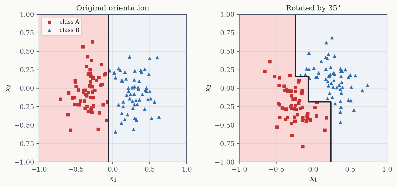
A shallow tree produces a coarse staircase that underfits; a deep one places a leaf around almost every point and fits the noise. A further peculiarity is that, because splits are axis-aligned, trees are sensitive to the orientation of the data: a boundary that runs diagonally through the feature space must be approximated by many small steps. Rotating the features (for example with a PCA pre-processing step) can yield a simpler, better tree.
A single decision tree is rarely competitive on its own, but it is the building block of two very effective models in this chapter – the random forest and gradient boosting – which combine many trees to overcome the high variance of an individual tree.
7.3 Ensemble Methods: Bagging vs. Boosting
An ensemble combines many individual models (“learners”) into a single, stronger meta-model. The simplest ensemble is voting: several different models are trained on the same data and their outputs combined by majority vote (classification) or averaging (regression). More powerful ensembles instead combine many copies of the same kind of model, each exposed to slightly different data. Two complementary strategies of this kind exist, distinguished by the type of learner they combine.
Bagging (bootstrap aggregating) combines strong learners trained in parallel. Each learner is fitted to a different bootstrap resample of the training data and is deliberately flexible – a deep decision tree with low bias but high variance. Each resample is drawn with replacement, so some training points recur and others are omitted, and every learner sees a slightly different dataset. Averaging the predictions (or taking a majority vote) then reduces the variance. The random forest (described next) is the canonical example: many deep trees, each grown on a resampled dataset, combined by averaging.
Boosting combines weak learners trained in series. Each learner is deliberately inflexible – a shallow decision tree, or “stump”, with high bias. Rather than resampling the data, each new learner is trained to correct the errors of its predecessors. Typically hundreds or thousands of weak trees are stacked. Gradient boosting is the principal member of this family.
| Bagging (random forest) | Boosting (gradient boosting) | |
|---|---|---|
| Learners run | in parallel | in series |
| Base learner | deep tree (strong, low bias) | shallow tree (weak, high bias) |
| Training data | bootstrap resamples | residuals of previous models |
| Combination | average / majority vote | weighted sum |
| Reduces mainly | variance | bias |
7.3.1 Random Forest
A random forest is the most widely used bagging ensemble. It builds on bagged decision trees with one additional source of randomness: at every split, only a random subset of the features is considered as candidates, rather than all of them. Bootstrap resampling already makes the trees differ; restricting the features at each split decorrelates them further, because no single dominant feature can sit at the top of every tree. Averaging a collection of diverse, individually high-variance trees yields a model with substantially lower variance while retaining their low bias.
The two principal hyperparameters are the number of trees – more trees never reduce accuracy and only cost computation, so the default of around 100 is usually adequate – and max_features, the size of the feature subset, which is lowered for high-dimensional data. The defaults are generally reasonable, which is part of why random forests are such dependable off-the-shelf models.
The widget below illustrates the variance-reduction mechanism in one dimension. Each thin curve is a deep tree fitted to its own bootstrap resample; the bold curve is their average. A single tree is jagged and overfits, but as trees are added their average converges to a smooth, stable estimate.
#| '!! shinylive warning !!': |
#|   shinylive does not work in self-contained HTML documents.
#|   Please set `embed-resources: false` in your metadata.
#| standalone: true
#| viewerHeight: 640

from shiny import App, render, ui
import numpy as np
import matplotlib.pyplot as plt
import matplotlib

matplotlib.rcParams.update({
    "font.family": "serif",
    "figure.facecolor": "#fafaf7",
    "axes.facecolor": "#fafaf7",
    "axes.grid": True,
    "grid.alpha": 0.3,
})

BLUE = "#2b6cb0"
RED = "#c53030"
PURPLE = "#805ad5"

np.random.seed(21)
n = 60
x_data = np.linspace(-3, 3, n)
y_true = np.sin(1.2 * x_data) + 0.3 * x_data
y_data = y_true + np.random.normal(0, 0.3, n)


def build_tree(x, y, depth, max_depth, min_samples=1):
    node = {"value": float(y.mean())}
    if depth >= max_depth or len(y) < 2 * min_samples:
        return node
    order = np.argsort(x)
    xs, ys = x[order], y[order]
    nn = len(ys)
    csum = np.cumsum(ys)
    csum2 = np.cumsum(ys ** 2)
    total, total2 = csum[-1], csum2[-1]
    i = np.arange(1, nn)
    left_sum, left_n = csum[:-1], i
    right_sum, right_n = total - left_sum, nn - i
    left_sse = csum2[:-1] - left_sum ** 2 / left_n
    right_sse = (total2 - csum2[:-1]) - right_sum ** 2 / right_n
    sse = left_sse + right_sse
    valid = (xs[1:] != xs[:-1]) & (left_n >= min_samples) & (right_n >= min_samples)
    if not valid.any():
        return node
    sse = np.where(valid, sse, np.inf)
    k = int(np.argmin(sse))
    thr = 0.5 * (xs[k] + xs[k + 1])
    mask = x <= thr
    node["thr"] = thr
    node["left"] = build_tree(x[mask], y[mask], depth + 1, max_depth, min_samples)
    node["right"] = build_tree(x[~mask], y[~mask], depth + 1, max_depth, min_samples)
    return node


def predict_tree(node, x):
    if "thr" not in node:
        return np.full(x.shape, node["value"])
    out = np.empty(x.shape)
    mask = x <= node["thr"]
    out[mask] = predict_tree(node["left"], x[mask])
    out[~mask] = predict_tree(node["right"], x[~mask])
    return out


app_ui = ui.page_fluid(
    ui.layout_columns(
        ui.input_slider("n_trees", "Number of trees", min=1, max=50, value=1, step=1),
        ui.input_slider("depth", "Tree depth", min=2, max=10, value=8, step=1),
    ),
    ui.output_plot("rf_plot"),
)


def server(input, output, session):
    @render.plot
    def rf_plot():
        n_trees = input.n_trees()
        depth = input.depth()
        xs = np.linspace(-3, 3, 500)

        rng = np.random.default_rng(7)
        preds = np.empty((n_trees, xs.size))
        preds_tr = np.empty((n_trees, n))
        for t in range(n_trees):
            idx = rng.integers(0, n, n)
            tree = build_tree(x_data[idx], y_data[idx], 0, depth)
            preds[t] = predict_tree(tree, xs)
            preds_tr[t] = predict_tree(tree, x_data)
        avg = preds.mean(0)
        mse = float(np.mean((y_data - preds_tr.mean(0)) ** 2))

        fig, ax = plt.subplots(figsize=(6, 4.4))
        ax.set_xlim(-3.1, 3.1)
        ax.set_ylim(-2.4, 2.4)
        for t in range(n_trees):
            ax.plot(xs, preds[t], color=PURPLE, linewidth=0.6, alpha=0.25)
        ax.plot(xs, np.sin(1.2 * xs) + 0.3 * xs, color="#999",
                linewidth=1.5, linestyle="--", label="True function")
        ax.plot(xs, avg, color=RED, linewidth=2.6, label="Forest average")
        ax.scatter(x_data, y_data, color=BLUE, s=20, alpha=0.7, zorder=5)
        ax.text(0.02, 0.97, f"ensemble train MSE = {mse:.3f}",
                transform=ax.transAxes, va="top", fontsize=10, fontweight="bold",
                color="#333", bbox=dict(boxstyle="round,pad=0.4", facecolor="white", edgecolor="#ddd"))
        ax.legend(loc="lower right", fontsize=9, framealpha=0.9)
        ax.set_xlabel("x")
        ax.set_ylabel("y")
        fig.tight_layout()
        return fig


app = App(app_ui, server)
7.3.2 Gradient Boosting
The central idea of gradient boosting is to train each new tree on the residuals of the previous ones, so that every tree learns a correction to the accumulated prediction.
- The first model \(h_1\) is fitted to the original data. As a weak learner, it captures only the coarse trend.
- The second model \(h_2\) is fitted not to the targets but to the residuals \(\mathbf{y} - \hat{\mathbf{y}}\) remaining after \(h_1\).
- The third model \(h_3\) is fitted to the residuals remaining after \(h_1\) and \(h_2\), and so on.
Because each tree only corrects the errors of its predecessors, the residuals shrink at every stage. The final prediction is the (weighted) sum of all trees:
\[ \hat{f}(\mathbf{x}) = \sum_{i} \eta\, h_i(\mathbf{x}). \]
The factor \(\eta\) is the learning rate, which scales down the contribution of each tree so that no single model dominates. Small learning rates (typically \(0.01\)–\(0.1\)) require more trees but improve generalization, analogous to a small step size in gradient descent. The term “gradient” in gradient boosting reflects this correspondence: for the squared-error loss the residual equals the negative gradient of the loss with respect to the prediction, so fitting the residuals is a form of functional gradient descent.
The widget below fits a gradient-boosting ensemble of shallow regression trees implemented from scratch. Varying the number of trees, the learning rate, and the tree depth illustrates how the piecewise-constant fit tightens around the data.
#| '!! shinylive warning !!': |
#|   shinylive does not work in self-contained HTML documents.
#|   Please set `embed-resources: false` in your metadata.
#| standalone: true
#| viewerHeight: 600

from shiny import App, render, ui
import numpy as np
import matplotlib.pyplot as plt
import matplotlib

matplotlib.rcParams.update({
    "font.family": "serif",
    "figure.facecolor": "#fafaf7",
    "axes.facecolor": "#fafaf7",
    "axes.grid": True,
    "grid.alpha": 0.3,
})

BLUE = "#2b6cb0"
RED = "#c53030"
ORANGE = "#e8833a"
GREEN = "#276749"
PURPLE = "#805ad5"

# Data: a curved, noisy target
np.random.seed(7)
n = 70
x_data = np.linspace(-2, 2, n)
y_true = 0.45 * x_data**2 + 0.4 * np.sin(3 * x_data)
y_data = y_true + np.random.uniform(-0.25, 0.25, n)


def build_tree(x, y, depth, max_depth, min_samples=3):
    """Greedy 1-D regression tree via vectorized split search."""
    node = {"value": float(y.mean())}
    if depth >= max_depth or len(y) < 2 * min_samples:
        return node
    order = np.argsort(x)
    xs, ys = x[order], y[order]
    nn = len(ys)
    csum = np.cumsum(ys)
    csum2 = np.cumsum(ys**2)
    total, total2 = csum[-1], csum2[-1]
    i = np.arange(1, nn)
    left_sum, left_n = csum[:-1], i
    right_sum, right_n = total - left_sum, nn - i
    left_sse = csum2[:-1] - left_sum**2 / left_n
    right_sse = (total2 - csum2[:-1]) - right_sum**2 / right_n
    sse = left_sse + right_sse
    valid = (xs[1:] != xs[:-1]) & (left_n >= min_samples) & (right_n >= min_samples)
    if not valid.any():
        return node
    sse = np.where(valid, sse, np.inf)
    k = int(np.argmin(sse))
    thr = 0.5 * (xs[k] + xs[k + 1])
    mask = x <= thr
    node["thr"] = thr
    node["left"] = build_tree(x[mask], y[mask], depth + 1, max_depth, min_samples)
    node["right"] = build_tree(x[~mask], y[~mask], depth + 1, max_depth, min_samples)
    return node


def predict_tree(node, x):
    if "thr" not in node:
        return np.full(x.shape, node["value"])
    out = np.empty(x.shape)
    mask = x <= node["thr"]
    out[mask] = predict_tree(node["left"], x[mask])
    out[~mask] = predict_tree(node["right"], x[~mask])
    return out


app_ui = ui.page_fluid(
    ui.layout_columns(
        ui.input_slider("n_est", "Number of trees", min=1, max=200, value=3, step=1),
        ui.input_slider("lr", "Learning rate", min=0.02, max=1.0, value=1.0, step=0.02),
        ui.input_slider("depth", "Tree depth", min=1, max=4, value=1, step=1),
    ),
    ui.output_plot("gb_plot"),
)


def server(input, output, session):
    @render.plot
    def gb_plot():
        n_est = input.n_est()
        lr = input.lr()
        depth = input.depth()

        # Fit gradient boosting on residuals
        pred = np.zeros_like(y_data)
        for _ in range(n_est):
            resid = y_data - pred
            tree = build_tree(x_data, resid, 0, depth)
            pred = pred + lr * predict_tree(tree, x_data)

        # Smooth curve for plotting (re-fit cumulatively)
        xs_fit = np.linspace(-2, 2, 400)
        pred_fit = np.zeros_like(xs_fit)
        pred_tr = np.zeros_like(y_data)
        for _ in range(n_est):
            resid = y_data - pred_tr
            tree = build_tree(x_data, resid, 0, depth)
            pred_tr = pred_tr + lr * predict_tree(tree, x_data)
            pred_fit = pred_fit + lr * predict_tree(tree, xs_fit)

        mse = float(np.mean((y_data - pred) ** 2))

        fig, ax = plt.subplots(figsize=(6, 4.2))
        ax.set_xlim(-2.1, 2.1)
        ax.set_ylim(-0.6, 2.6)
        ax.plot(xs_fit, 0.45 * xs_fit**2 + 0.4 * np.sin(3 * xs_fit),
                color="#999", linewidth=1.5, linestyle="--", label="True function")
        ax.plot(xs_fit, pred_fit, color=RED, linewidth=2.5, label="Ensemble prediction")
        ax.scatter(x_data, y_data, color=BLUE, s=22, alpha=0.7, zorder=5)
        ax.text(0.02, 0.97, f"train MSE = {mse:.4f}",
                transform=ax.transAxes, va="top", fontsize=10, fontweight="bold",
                color="#333", bbox=dict(boxstyle="round,pad=0.4", facecolor="white", edgecolor="#ddd"))
        ax.legend(loc="upper right", fontsize=9, framealpha=0.9)
        ax.set_xlabel("x")
        ax.set_ylabel("y")
        fig.tight_layout()
        return fig


app = App(app_ui, server)
A small number of depth-1 stumps produces a crude staircase that underfits the curve, and adding trees refines it. The two main knobs interact: a large learning rate combined with many trees begins to fit the noise, whereas a small learning rate requires many more trees to reach the same fit. For this reason the learning rate and the number of trees are tuned jointly and selected via cross-validation or a train-validation split.
The number of trees can also be chosen automatically through early stopping. As trees are added, the training error continues to decrease but the validation error flattens and eventually begins to rise. Early stopping halts training once the validation error ceases to improve over a given number of iterations.
7.4 The Kernel Trick
Kernel methods address non-linearity from a different direction. The objective is the same as in polynomial regression – to fit a linear model in a higher-dimensional, enlarged feature space – but without incurring the cost of constructing that space.
Conceptually, the procedure is:
- begin with data that is not linearly separable in its original space;
- apply a mapping \(\phi(\mathbf{x})\) that lifts it into a higher-dimensional space in which it is linearly separable;
- fit a linear model in that space; and
- project the result back, where it appears as a curved boundary.
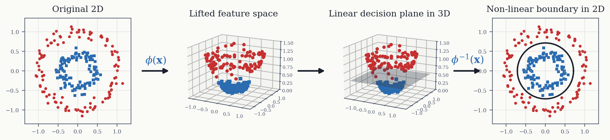
Constructing \(\phi(\mathbf{x})\) explicitly is the costly step. The kernel trick is the observation that, for an appropriate class of models, the lifted features appear only inside dot products \(\phi(\mathbf{x}^{(i)})^\top \phi(\mathbf{x}^{(j)})\), and that these dot products can frequently be computed directly from the original features by an inexpensive kernel function, without ever forming \(\phi(\mathbf{x})\).
7.4.1 Kernel ridge regression
To illustrate how a model can be expressed purely in terms of dot products, consider ridge regression. Its usual primal form predicts using one weight per feature,
\[ \hat{y}(\mathbf{x}^{(j)}) = \mathbf{w}^\top \mathbf{x}^{(j)}. \]
The same model can be rewritten in dual form, with one weight \(\alpha_i\) per training point, so that the prediction is a weighted sum of similarities to the training data:
\[ \hat{y}(\mathbf{x}^{(j)}) = \sum_{i=1}^{n} \alpha_i\, \kappa\!\left(\mathbf{x}^{(i)}, \mathbf{x}^{(j)}\right) \;\overset{\substack{\text{linear}\\\text{kernel}}}{=} \sum_{i=1}^{n} \alpha_i\, \mathbf{x}^{(i)\top} \mathbf{x}^{(j)}. \]
Here \(\kappa\) is the kernel function. For a linear model it is simply the dot product, i.e. the projection of each training-point vector onto the query vector. The two forms are connected by \(\mathbf{w} = \mathbf{X}^\top \boldsymbol{\alpha}\), and the dual weights have a closed-form solution that parallels ordinary ridge regression:
\[ \boldsymbol{\alpha} = (\mathbf{K} + \lambda \mathbf{I})^{-1}\, \mathbf{y}, \qquad \mathrm{K}_{i,j} = \kappa\!\left(\mathbf{x}^{(i)}, \mathbf{x}^{(j)}\right). \]
The matrix \(\mathbf{K}\) is the kernel matrix (or Gram matrix), collecting the kernel similarities between all pairs of training points. The regularization parameter \(\lambda\) plays the same role as in ridge regression; in the scikit-learn KernelRidge estimator it is exposed as alpha, with larger values producing a smoother fit.
The significance of the dual form is that it does not require the kernel to be a dot product. Any valid kernel can be substituted to obtain a non-linear model, while the fitting equations remain unchanged.
7.4.2 A worked polynomial kernel
The efficiency of a kernel function over the explicit lift can be demonstrated with the second-degree polynomial lift in two dimensions,
\[ \varphi(\mathbf{x}) = \varphi\!\left(\begin{pmatrix} x_1 \\ x_2 \end{pmatrix}\right) = \begin{pmatrix} x_1^2 \\ \sqrt{2}\, x_1 x_2 \\ x_2^2 \end{pmatrix}. \]
Computing the dot product of two lifted vectors directly gives
\[ \varphi(\mathbf{a})^\top \varphi(\mathbf{b}) = a_1^2 b_1^2 + 2 a_1 b_1 a_2 b_2 + a_2^2 b_2^2 = (a_1 b_1 + a_2 b_2)^2 = \left(\mathbf{a}^\top \mathbf{b}\right)^2. \]
The operation in the three-dimensional lifted space reduces to squaring a dot product in the original two-dimensional space. This is precisely the kernel function \(\kappa(\mathbf{a}, \mathbf{b}) = (\mathbf{a}^\top \mathbf{b})^2\). The saving increases sharply with input dimension and polynomial degree: the lifted space may contain thousands of coordinates, but the kernel always operates in the original dimension.
7.4.3 Important kernel functions
Any function that can be written as an inner product in some lifted space is a valid kernel; formally, it must satisfy Mercer’s condition. The most common kernels are:
| Name | \(\kappa(\mathbf{x}^{(i)}, \mathbf{x}^{(j)})\) | Parameters |
|---|---|---|
| Linear | \(\mathbf{x}^{(i)\top}\mathbf{x}^{(j)}\) | – |
| Polynomial | \(\left(\gamma\, \mathbf{x}^{(i)\top}\mathbf{x}^{(j)} + r\right)^{d}\) | \(d\) degree, \(r\) offset, \(\gamma\) scale |
| Radial basis function (RBF / Gaussian) | \(\exp\!\left(-\gamma \lVert \mathbf{x}^{(i)} - \mathbf{x}^{(j)} \rVert_2^2\right)\) | \(\gamma\) “inverse length” |
| Exponential | \(\exp\!\left(-\gamma \lVert \mathbf{x}^{(i)} - \mathbf{x}^{(j)} \rVert_2\right)\) | \(\gamma\) “inverse length” |
| Laplacian | \(\exp\!\left(-\gamma \lVert \mathbf{x}^{(i)} - \mathbf{x}^{(j)} \rVert_1\right)\) | \(\gamma\) “inverse length” |
| Matérn 3/2 | \(\left(1 + \gamma \lVert \mathbf{x}^{(i)} - \mathbf{x}^{(j)} \rVert_2\right)\exp\!\left(-\gamma \lVert \mathbf{x}^{(i)} - \mathbf{x}^{(j)} \rVert_2\right)\) | \(\gamma\) “inverse length” |
| Sigmoid | \(\tanh\!\left(\gamma\, \mathbf{x}^{(i)\top}\mathbf{x}^{(j)} + r\right)\) | \(\gamma\), \(r\) |
The polynomial kernel reduces to the worked example above for \(d=2\), \(r=0\), \(\gamma=1\).
The kernel families differ in how training points contribute to a prediction. The linear kernel weights each training point by the projection of its vector onto the query point, so the contribution depends on the dot product irrespective of distance. The RBF/Gaussian kernel instead weights each training point by a similarity that decays exponentially with distance, so only nearby training points contribute appreciably. The choice of kernel therefore encodes an assumption about the roughness of the structure–property landscape: the Matérn and exponential kernels decay more rapidly than the Gaussian and are correspondingly more “short-sighted”, which suits rougher landscapes.
7.4.4 Interactive example: kernels and regularization
The widget fits a kernel ridge regression from scratch. Not all kernels have all parameters: the linear kernel has none, the RBF kernel has \(\gamma\), and the polynomial kernel has both \(\gamma\) and its degree. The regularization \(\lambda\) applies in every case. The RBF kernel makes the near-/short-sightedness explicit: a small \(\gamma\) yields broad, smooth curves (far-sighted), and a large \(\gamma\) yields narrow, oscillatory ones (near-sighted). Increasing \(\lambda\) smooths the fit by shrinking the dual weights.
#| '!! shinylive warning !!': |
#|   shinylive does not work in self-contained HTML documents.
#|   Please set `embed-resources: false` in your metadata.
#| standalone: true
#| viewerHeight: 640

from shiny import App, render, ui
import numpy as np
import matplotlib.pyplot as plt
import matplotlib

matplotlib.rcParams.update({
    "font.family": "serif",
    "figure.facecolor": "#fafaf7",
    "axes.facecolor": "#fafaf7",
    "axes.grid": True,
    "grid.alpha": 0.3,
})

BLUE = "#2b6cb0"
RED = "#c53030"
ORANGE = "#e8833a"
GREEN = "#276749"
PURPLE = "#805ad5"

np.random.seed(3)
n = 18
x_train = np.sort(np.random.uniform(-3, 3, n))
y_clean = np.sin(1.3 * x_train) + 0.3 * x_train
y_train = y_clean + np.random.uniform(-0.25, 0.25, n)


def kernel(A, B, ktype, gamma, degree):
    """A: (n,1), B: (m,1) -> (n,m) kernel matrix."""
    if ktype == "Linear":
        return A @ B.T
    if ktype == "Polynomial":
        return (gamma * (A @ B.T) + 1.0) ** degree
    # RBF
    d2 = (A - B.T) ** 2
    return np.exp(-gamma * d2)


app_ui = ui.page_fluid(
    ui.layout_columns(
        ui.input_radio_buttons("ktype", "Kernel",
                               choices=["RBF", "Polynomial", "Linear"], selected="RBF"),
        # gamma and degree do not appear in every kernel, so each slider is only
        # shown for the kernels whose definition actually contains it. The linear
        # kernel has no parameters at all.
        ui.panel_conditional(
            "input.ktype !== 'Linear'",
            ui.input_slider("gamma", "Kernel parameter (gamma)", min=0.05, max=5.0, value=1.0, step=0.05),
        ),
        ui.input_slider("lam", "Regularization (lambda)", min=0.001, max=2.0, value=0.05, step=0.001),
        ui.panel_conditional(
                "input.ktype === 'Polynomial'",
                ui.input_slider("degree", "Polynomial degree", min=2, max=6, value=3, step=1),
            ),
    ),
    ui.output_plot("krr_plot"),
)


def server(input, output, session):
    @render.plot
    def krr_plot():
        ktype = input.ktype()
        gamma = input.gamma() or 1.0
        lam = input.lam()
        degree = input.degree() or 3

        Xtr = x_train[:, None]
        K = kernel(Xtr, Xtr, ktype, gamma, degree)
        alpha = np.linalg.solve(K + lam * np.eye(n), y_train)

        xs = np.linspace(-3.4, 3.4, 400)
        Ks = kernel(xs[:, None], Xtr, ktype, gamma, degree)
        y_pred = Ks @ alpha
        mse = float(np.mean((y_train - kernel(Xtr, Xtr, ktype, gamma, degree) @ alpha) ** 2))

        fig, ax = plt.subplots(figsize=(6, 4.2))
        ax.set_xlim(-3.5, 3.5)
        ax.set_ylim(-2.5, 2.5)

        # Individual weighted kernel basis functions (RBF only, for intuition)
        if ktype == "RBF":
            for xi, ai in zip(x_train, alpha):
                ax.plot(xs, ai * np.exp(-gamma * (xs - xi) ** 2),
                        color=PURPLE, linewidth=0.7, alpha=0.35)

        ax.plot(xs, np.sin(1.3 * xs) + 0.3 * xs, color="#999",
                linewidth=1.5, linestyle="--", label="True function")
        ax.plot(xs, np.clip(y_pred, -2.5, 2.5), color=RED, linewidth=2.5, label="KRR prediction")
        ax.scatter(x_train, y_train, color=BLUE, s=28, alpha=0.8, zorder=5)

        ax.text(0.02, 0.97, f"train MSE = {mse:.4f}",
                transform=ax.transAxes, va="top", fontsize=10, fontweight="bold",
                color="#333", bbox=dict(boxstyle="round,pad=0.4", facecolor="white", edgecolor="#ddd"))
        ax.legend(loc="lower right", fontsize=9, framealpha=0.9)
        ax.set_xlabel("x")
        ax.set_ylabel("y")
        fig.tight_layout()
        return fig


app = App(app_ui, server)
The thin purple curves (shown for the RBF kernel) are the individual weighted terms \(\alpha_i\, \kappa(\cdot, x^{(i)})\), and the red prediction is their sum. A very large \(\gamma\) collapses each term onto its own training point, producing a spiky overfit, whereas a large \(\lambda\) relaxes the fit toward a smooth, nearly flat line. The linear kernel can only represent a straight line, regardless of its parameters.
7.5 When to Use Which Model
The following guidance summarizes common practice:
- Decision trees are valued more for transparency and simplicity than for accuracy: a single shallow tree is directly interpretable.
- Random forests are excellent default models that work well with little or no tuning, tolerate mixed feature scales, and provide a built-in feature-importance estimate.
- Gradient boosting and kernel methods are reliable defaults for tabular chemical data. Gradient boosting in particular is consistently among the strongest performers on tabular benchmarks and competitions.
- Kernel methods are advantageous when a meaningful similarity measure is available for the data, including specialized kernels for fingerprints, molecular graphs, SMILES strings, and the SOAP descriptor. They also form the basis of Gaussian process regression, which is central to Bayesian optimization.
- Feed-forward neural networks on tabular data often require disproportionate effort relative to their benefit; their primary value lies in serving as the building block of graph and language models. They are the subject of the following chapter.
7.6 Summary
- Why go non-linear. Linear models are restricted to flat surfaces and hyperplane boundaries, which many chemical problems violate. The most direct fix, polynomial regression, enriches the features with higher-degree and cross terms — but the number of terms grows as \((m+d)!/(d!\,m!)\), so explicitly building that space quickly becomes infeasible and overfits readily.
- Decision trees partition the input space directly with a sequence of axis-aligned yes/no splits, giving a piecewise-constant surface. The greedy CART algorithm chooses each split to minimize the weighted impurity of the children — MSE for regression, Gini impurity for classification. Trees have low bias but high variance, so growth must be limited (chiefly by maximum depth), and because splits are axis-aligned they are sensitive to the orientation of the data.
- Ensembles combine many trees. Bagging trains strong learners (deep trees) in parallel on bootstrap resamples and averages them, reducing variance. Boosting trains weak learners (shallow stumps) in series, each fitted to the residuals of its predecessors, reducing bias.
- Random forests add a second source of randomness by considering only a random subset of features at each split which decorrelates the trees and improves the averaging. They need little tuning, which is much of their appeal.
- Gradient boosting sums trees scaled by a learning rate \(\eta\); small \(\eta\) needs more trees but generalizes better, so the two are tuned jointly, often with early stopping. For squared-error loss the residual is the negative gradient of the loss, which is where the name comes from.
- Kernel methods reach an enlarged feature space without ever constructing it. Written in dual form, ridge regression depends on the data only through dot products, which a kernel function \(\kappa\) can compute directly in the original space: the kernel trick. Fitting reduces to \(\boldsymbol{\alpha} = (\mathbf{K} + \lambda\mathbf{I})^{-1}\mathbf{y}\) with the kernel matrix \(\mathbf{K}\).
- The kernel encodes an assumption about the roughness of the structure–property landscape: the linear kernel weights training points by projection regardless of distance, while RBF, Matérn and exponential kernels decay with distance, the latter two more sharply and so better suited to rougher landscapes. Specialized kernels exist for fingerprints, graphs, SMILES and SOAP, and kernel methods underpin the Gaussian process regression used in Bayesian optimization.