---
title: "Physics-Based Simulation and Representations"
format:
html:
code-fold: true
toc: true
theme: cosmo
jupyter: python3
---
In data-driven chemistry, we start from a 2D molecular graph and make predictions based on available experimental data. A complementary route is to predict chemistry **from first principles**. We can achieve this by computing the molecular Hamiltonian as a function of the positions and charges of its nuclei and the number of electrons, and from that derive everything else: stable structures, reaction barriers, spectra, solubility, etc. This is the domain of physics-based simulation.
The appeal is obvious. If we can compute a property instead of measuring it, we can replace experiments that are too expensive, too slow, or too dangerous, and we can generate as much (clean, consistent) data as we are willing to pay for. The difficulty is equally obvious: solving the underlying physics exactly is computationally intractable for all but the smallest systems, so the whole field is built around a hierarchy of **approximations** that trade accuracy for cost.
In this chapter we will explain how simulation works and why it is hard: the potential energy surface, the Schrödinger equation, and the cost–accuracy hierarchy of methods (force fields, ML potentials, semi-empirical, DFT, correlated wavefunction methods). Then we will see how the *output* of simulation becomes a molecular representation for machine learning: quantum-chemical descriptors (charges, Fukui indices). Finally, we will present some descriptors that do not involve simulations but were inspired by physics to be data-efficient and descriptive (the Coulomb matrix, SOAP), which featurize 3D coordinates and atom types as input for machine-learning models.
## Predicting chemistry from first principles
### The potential energy surface
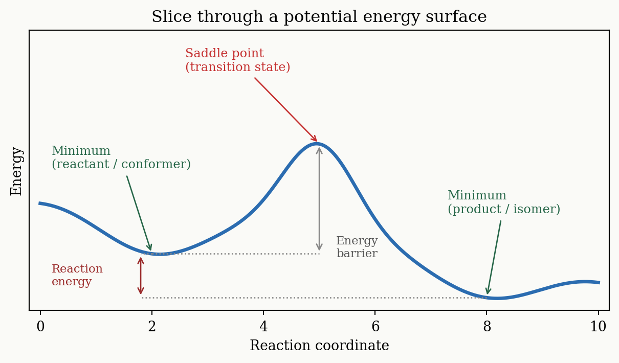
A molecule of $N$ atoms lives in a $3N$-dimensional space of nuclear coordinates. For every geometry $\mathbf{R} = (\mathbf{r}_1, \dots, \mathbf{r}_N)$ there is a single number — the electronic energy of that arrangement. The function mapping coordinates to energy,
$$
E = E(\mathbf{r}_1, \mathbf{r}_2, \dots, \mathbf{r}_N),
$$
is the **potential energy surface (PES)**. Almost all of chemistry can be read off the shape of this surface:
- **Minima** are stable structures — conformers, isomers, reactants, products. A molecule at rest sits in a minimum.
- A **first-order saddle point** along a reaction coordinate — a maximum *along the path* but a minimum in every direction perpendicular to it — is a **transition state**; the energy difference from a minimum to the connecting saddle point is a **reaction barrier**, which controls reaction *rates*.
- **Energy differences between minima** are reaction or conformational energies, which control *equilibria* and selectivity.
- **Free energies** can be obtained by simulating dynamics on the PES or from static picture under certain approximations.
The fundamental task of any simulation method is therefore to compute the energy at a given geometry — and, ideally, its derivatives. The first derivative with respect to coordinates gives the **forces** (used to optimize geometries and run molecular dynamics); the second derivatives give the **vibrational frequencies** (used for thermochemistry and IR spectra). Other properties are derivatives with respect to an **external field** rather than to the coordinates: the dipole moment and polarizability are the first and second derivatives of the energy with respect to an electric field, and NMR shieldings involve a magnetic field.
::: {.callout-note}
The PES is a high-dimensional object, but we usually visualize a 1D or 2D *slice* along the coordinate(s) that change during a process — e.g. a dihedral angle for a conformational change, or a forming/breaking bond length for a reaction.
:::
```{python}
#| label: fig-pes-slice
#| fig-cap: "A 1D slice through a potential energy surface along a reaction coordinate, with the key topographical features labeled."
import numpy as np
import matplotlib.pyplot as plt

plt.rcParams.update(
    {
        "font.family": "serif",
        "figure.facecolor": "#fafaf7",
        "axes.facecolor": "#fafaf7",
    }
)

np.random.seed(0)
x = np.linspace(0, 10, 500)
# A double-well with a barrier: reactant minimum, TS, product minimum.
# The linear tilt makes the product lie lower than the reactant (exergonic).
y = (
    0.6 * (x - 2.0) ** 2 * np.exp(-0.25 * (x - 2.0) ** 2)
    + 1.0 * np.exp(-1.2 * (x - 5.0) ** 2) * 2.2
    + 0.5 * (x - 8.0) ** 2 * np.exp(-0.25 * (x - 8.0) ** 2)
)
y = y - 0.18 * x
y = y - y.min()

r_i = np.argmin(np.abs(x - 2.0))  # reactant minimum
p_i = np.argmin(np.abs(x - 8.0))  # product minimum
ts_i = np.argmin(np.abs(x - 5.0))  # transition state

fig, ax = plt.subplots(figsize=(6.4, 3.8))
ax.plot(x, y, color="#2b6cb0", lw=2.5)

# Reactant minimum
ax.annotate(
    "Minimum\n(reactant / conformer)",
    xy=(2.0, y[r_i]),
    xytext=(0.2, 3.2),
    fontsize=9,
    color="#276749",
    ha="left",
    arrowprops=dict(arrowstyle="->", color="#276749"),
)
# Product minimum
ax.annotate(
    "Minimum\n(product / isomer)",
    xy=(8.0, y[p_i]),
    xytext=(7.3, 2.1),
    fontsize=9,
    color="#276749",
    ha="left",
    arrowprops=dict(arrowstyle="->", color="#276749"),
)
# Transition state
ax.annotate(
    "Saddle point\n(transition state)",
    xy=(5.0, y[ts_i]),
    xytext=(2.6, 5.6),
    fontsize=9,
    color="#c53030",
    ha="left",
    arrowprops=dict(arrowstyle="->", color="#c53030"),
)
# Barrier arrow (activation energy from the reactant level)
ax.plot([2.0, 5.0], [y[r_i], y[r_i]], ls=":", lw=1.0, color="#888888")
ax.annotate(
    "",
    xy=(5.0, y[ts_i]),
    xytext=(5.0, y[r_i]),
    arrowprops=dict(arrowstyle="<->", color="#888888"),
)
ax.text(
    5.3,
    0.5 * (y[ts_i] + y[r_i]) - 1.2,
    "Energy\nbarrier",
    fontsize=8.5,
    color="#555555",
    va="center",
)

# Reaction energy: difference between reactant and product minima (exergonic here)
de_x = 1.8
ax.plot([2.0, de_x], [y[r_i], y[r_i]], ls=":", lw=1.0, color="#888888")
ax.plot([8.0, de_x], [y[p_i], y[p_i]], ls=":", lw=1.0, color="#888888")
ax.annotate(
    "",
    xy=(de_x, y[p_i]),
    xytext=(de_x, y[r_i]),
    arrowprops=dict(arrowstyle="<->", color="#9b2c2c"),
)
ax.text(
    0.2,
    0.5 * (y[r_i] + y[p_i]),
    "Reaction\nenergy",
    fontsize=8.5,
    color="#9b2c2c",
    ha="left",
    va="center",
)

ax.set_xlabel("Reaction coordinate")
ax.set_ylabel("Energy")
ax.set_title("Slice through a potential energy surface")
ax.set_yticks([])
ax.set_ylim(-0.3, 6.6)
ax.margins(x=0.02)
plt.tight_layout()
plt.show()
```
### The Schrödinger equation
Where does the energy come from? In principle, from the time-independent **Schrödinger equation**,
$$
\hat{H}\,\Psi = E\,\Psi,
$$
where $\hat{H}$ is the Hamiltonian operator (kinetic energy of nuclei and electrons plus all the Coulomb interactions between them), $\Psi$ is the many-body wavefunction, and $E$ is the energy. The **Born–Oppenheimer approximation** lets us separate the fast electrons from the slow nuclei: we clamp the nuclei in place, solve for the electrons, and obtain the electronic energy at that geometry — which is exactly the PES.
The catch is that $\Psi$ depends on the coordinates of *all* the electrons simultaneously, and the electron–electron repulsion couples them all together. Solving the equation exactly scales exponentially with the number of electrons, so an exact solution is intractable for anything beyond a handful of atoms. Every practical method is a controlled approximation to this equation — and the choice of approximation is the central decision in any simulation.
## The cost–accuracy hierarchy of methods
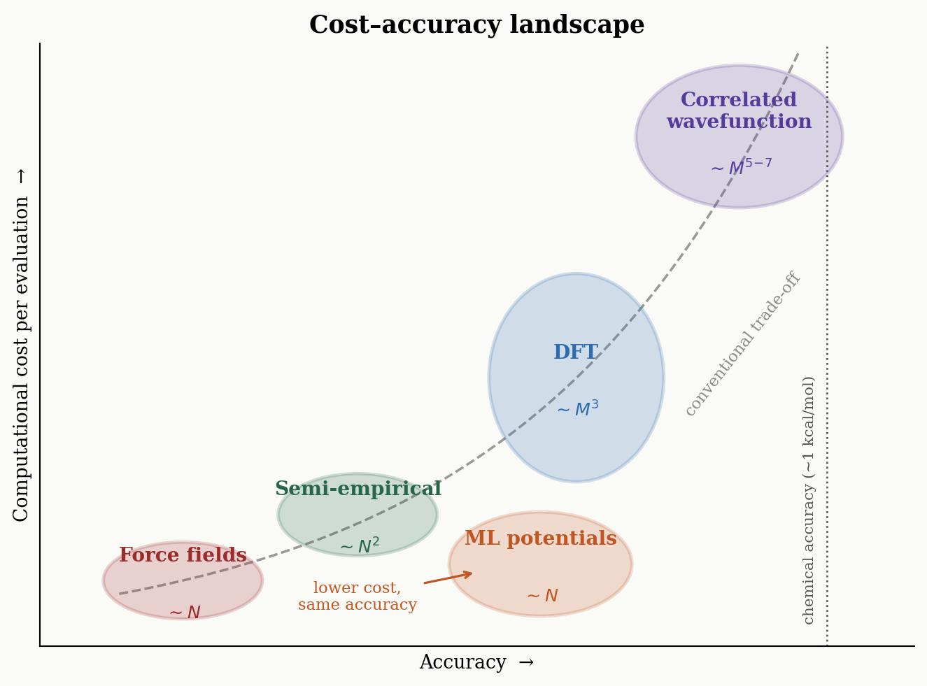
Methods for computing the energy form a hierarchy, from cheap-and-crude to expensive-and-exact:
| Family | Examples | Idea | Typical scaling |
|---|---|---|---|
| **Force fields** | MMFF94, UFF, GFN-FF | Classical springs and charges; *no electrons* | $\sim N$ |
| **ML potentials** | ANI-2x, MACE-OFF, AIMNet2 | Learn the PES from QM data | $\sim N$ |
| **Semi-empirical** | GFN2-xTB, PM6, AM1 | HF with most integrals replaced by parameters | $\sim N^2$ |
| **DFT** | B3LYP, r²SCAN-3c, ωB97X-3c | Energy as a functional of electron density | $\sim M^3$ |
| **Correlated wavefunction** | MP2, CCSD(T), Full CI | Explicit electron correlation; converges to exact | $M^5$ – $M^7$ |
Here $N$ is the number of atoms and $M$ the number of **basis functions** (roughly proportional to the number of electrons in the system). **Force fields** ignore electrons entirely: the energy is a sum of classical terms for bond stretches, angle bends, torsions, van der Waals, and electrostatics, with parameters fitted to experiment or to higher-level calculations. **Correlated wavefunction** methods, at the other extreme, treat electron correlation explicitly and converge to the exact answer (Full CI) as the basis set and the level of electron correlation increase.
### Computational scaling is the cost driver
The reason the hierarchy exists at all is **computational scaling** — how the cost grows with system size. The exponents are brutal for the accurate methods:
- Hartree–Fock (HF): $\approx M^4$
- MP2: $\approx M^5$
- CISD: $\approx M^6$
- CCSD(T) (the "gold standard"): $\approx M^7$
- Semi-empirical: $\approx N^2$
- DFT (Kohn–Sham): $\approx M^3$
An $M^7$ scaling means that doubling the system size makes the calculation $2^7 = 128$ times more expensive. This is why CCSD(T) is reserved for small molecules, DFT is the everyday workhorse, and force fields / ML potentials (which scale roughly *linearly* with the number of atoms thanks to distance cutoffs) are the only option for proteins and materials. Note that these exponents describe how cost *grows* with system size, not the absolute cost of a given calculation. Force fields and ML potentials share the same $\sim N$ scaling, but that does not make them equally fast: evaluating a classical force field is orders of magnitude cheaper per atom than evaluating a neural network, so force fields remain the choice when very long simulations are needed.
```{python}
#| label: fig-cost-hierarchy
#| fig-cap: "The cost–accuracy hierarchy of electronic-structure methods. The classical families trace a trade-off curve along which cost explodes as accuracy improves (note the large cost jump from DFT to coupled cluster, and the wide spread in DFT cost across functionals). ML potentials break the curve, reaching nearly DFT-level accuracy at close to force-field cost."
import numpy as np
import matplotlib.pyplot as plt
from matplotlib.patches import Ellipse

plt.rcParams.update({
    "font.family": "serif",
    "figure.facecolor": "#fafaf7",
    "axes.facecolor": "#fafaf7",
})

fig, ax = plt.subplots(figsize=(7.0, 5.2))
ax.set_xlim(0, 11)
ax.set_ylim(0, 11)

# Trade-off frontier: cost explodes as we demand more accuracy (accuracy on x, cost on y).
A, B = 3.52, 1.16
acc = np.linspace(1.0, 9.55, 200)
ax.plot(acc, np.exp((acc - B) / A), ls="--", lw=1.3, color="#999999", zorder=1)
ax.text(8.85, 5.5, "conventional trade-off", fontsize=8.5, color="#888888",
        rotation=52, rotation_mode="anchor", ha="center", va="center")

# (name, scaling, cx=accuracy, cy=cost, width, height, color)
# Ellipse height = spread in cost: small for FF/semi-empirical, large for DFT (functionals vary widely).
families = [
    ("Force fields",          r"$\sim N$",        1.8, 1.2, 2.0, 1.4, "#9b2c2c"),
    ("Semi-empirical",        r"$\sim N^2$",      4.0, 2.4, 2.0, 1.5, "#276749"),
    ("DFT",                   r"$\sim M^3$",      6.75, 4.9, 2.2, 3.8, "#2b6cb0"),
    ("Correlated\nwavefunction", r"$\sim M^{5\!-\!7}$", 8.8, 9.3, 2.6, 2.6, "#553c9a"),
    ("ML potentials",         r"$\sim N$",        6.3, 1.5, 2.3, 1.9, "#c05621"),
]

for name, scale, cx, cy, w, h, color in families:
    ax.add_patch(Ellipse((cx, cy), w, h, facecolor=color, alpha=0.20,
                         edgecolor=color, lw=1.8, zorder=2))
    ax.text(cx, cy + 0.45, name, ha="center", va="center", fontsize=10.5,
            fontweight="bold", color=color, zorder=3)
    ax.text(cx, cy - 0.6, scale, ha="center", va="center", fontsize=9.5,
            color=color, fontstyle="italic", zorder=3)

# ML potentials sit far below the curve: near-DFT accuracy at a fraction of the cost
ax.annotate("lower cost,\nsame accuracy", xy=(5.5, 1.35), xytext=(4.0, 0.9),
            fontsize=8.5, color="#c05621", ha="center", va="center",
            arrowprops=dict(arrowstyle="->", color="#c05621", lw=1.2))

# Chemical-accuracy guide line (now vertical)
ax.axvline(9.9, ls=":", lw=1.0, color="#555555")
ax.text(9.6, 0.4, "chemical accuracy (~1 kcal/mol)", rotation=90, fontsize=8,
        color="#555555", va="bottom", ha="left")

ax.set_xlabel("Accuracy  →", fontsize=10)
ax.set_ylabel("Computational cost per evaluation  →", fontsize=10)
ax.set_xticks([])
ax.set_yticks([])
for spine in ("top", "right"):
    ax.spines[spine].set_visible(False)
ax.set_title("Cost–accuracy landscape", fontsize=13, fontweight="bold")
plt.tight_layout()
plt.show()
```
### Bending the scaling curve
The exponents above are only the *nominal* scalings. Much of modern method development goes into beating them without sacrificing accuracy, which effectively shifts a method leftward in the cost–accuracy landscape.
::: {.callout-note collapse="true"}
## How the scaling is beaten (optional)
The most expensive quantities in a calculation are often nearly redundant or strongly local. **Density fitting / resolution-of-the-identity (RI)** and **chain-of-spheres exchange (COSX)** rewrite the costly electron-repulsion integrals of DFT in a far cheaper form, usually with negligible error. **Local correlation methods** such as DLPNO-CCSD(T) exploit the short-rangedness of electron correlation to confine the expensive coupled-cluster work to localized orbital pairs, bringing the nominal $M^7$ scaling down toward near-linear while staying close to gold-standard accuracy.
:::
## DFT and the functional zoo
Density functional theory (DFT) is the dominant method in practical computational chemistry because its $\sim M^3$ scaling buys a lot of accuracy per CPU hour. Its foundation is the **Hohenberg–Kohn theorem**: the ground-state electron density $\rho(\mathbf{r})$ — a function of just three spatial coordinates, no matter how many electrons — fully determines the energy and all properties of the system. We no longer need the full many-electron wavefunction.
This does not, however, make DFT a purely density-based method in practice. Because the kinetic energy is not known accurately as a functional of the density alone, most of DFT implementations are **Kohn–Sham DFT**, which reintroduces a set of one-electron orbitals to evaluate it. Those orbitals bring back integrals over basis functions, so the formal cost is $M^3$–$M^4$ rather than anything like the cost of working with a three-dimensional density.
In Kohn–Sham DFT the energy is written as
$$
E_{\text{DFT}}[\rho] = T_{\text{S}}[\rho] + E_{\text{ne}}[\rho] + J[\rho] + E_{\text{xc}}[\rho],
$$
where $T_{\text{S}}$ is the kinetic energy of non-interacting electrons, $E_{\text{ne}}$ the nuclear–electron attraction, and $J$ the classical Coulomb repulsion of the density with itself. The first three terms are well-behaved and known exactly. The trouble is the last term, the **exchange–correlation functional** $E_{\text{xc}}[\rho]$, which sweeps up all the quantum subtleties (exchange and electron correlation) into one object whose exact form is *unknown*. Every DFT calculation therefore uses an *approximation* to $E_{\text{xc}}$ — a **density functional approximation (DFA)**.
### Jacob's ladder
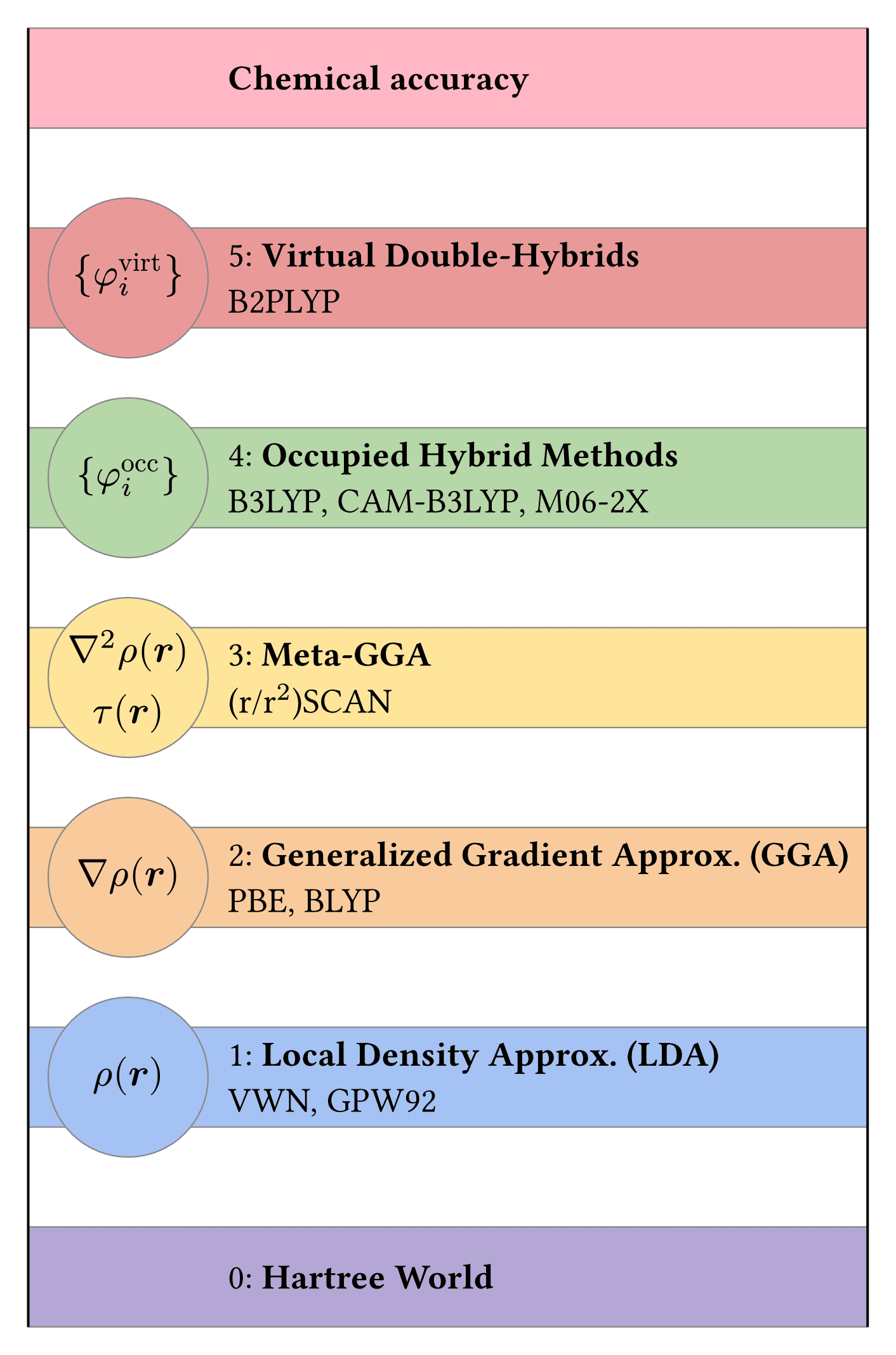
The DFAs are organized into rungs of increasing sophistication, cost, and (on average) accuracy — a hierarchy known as **Jacob's ladder**, climbing from the "Hartree hell" of crude approximations toward the "heaven of chemical accuracy":
1. **LDA** — uses only the local density $\rho(\mathbf{r})$.
2. **GGA** — adds the density gradient $\nabla\rho(\mathbf{r})$.
3. **meta-GGA** — adds the kinetic-energy density $\tau(\mathbf{r})$, or equivalently the density Laplacian $\nabla^2\rho(\mathbf{r})$.
4. **Hybrid** — mixes in a fraction of exact (Hartree–Fock) exchange; often the best accuracy/cost compromise.
5. **Double-hybrid** — adds MP2-like correlation; most accurate, most expensive.
{#fig-jacobs-ladder width=52%}
Crucially, **no one knows the exact functional**, and a higher rung is only better *on average* for lower rungs of the ladder. Hundreds of functionals exist (benchmark studies such as @goerigk2019zoo compare ~100 of them), and the best choice depends on your system and property. The practical rule is to **test for your use case** rather than trust a ranking blindly.
### Absolute values, error cancellation, and relative ranking
A theme that runs through all of computational chemistry: **absolute energies are extremely hard to compute accurately.** The total electronic energy of even a small molecule is hundreds or thousands of kcal/mol, and getting it right to "chemical accuracy" (~1 kcal/mol) in absolute terms is essentially hopeless with affordable methods. We almost never need the absolute number, though. Two quite different things rescue us, and it is worth keeping them apart — they are often lumped together under the single label "error cancellation".
**1. Error cancellation (in narrow sense).** What matters chemically is usually a *difference* between two species computed the same way: a reaction energy (product − reactant) or a barrier (transition state − reactant). If both species carry a similar systematic error, that error largely subtracts out of the difference, and the computed difference is far more accurate than either absolute energy behind it. This works best when the two species are genuinely similar: same number and type of atoms, similar bonding, same basis set and functional. It works badly when they are not — which is why reactions that change the number of bonds of a given type, or the spin state, or the charge, are much harder than a conformer gap. So **relative energies are more accessible than absolute ones, but they are not automatically easy**; the cancellation has to be earned by comparing like with like.
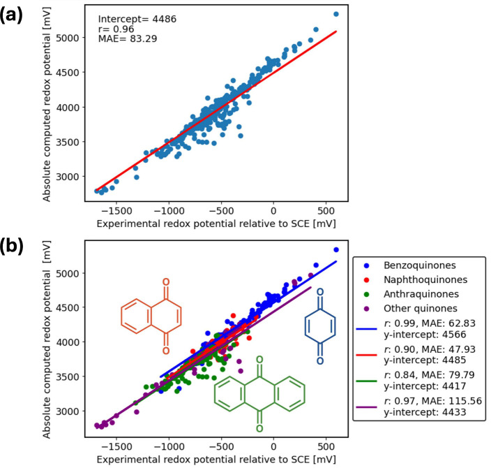
**2. Trend preservation, i.e. relative ranking.** A separate and weaker claim: even when nothing cancels, a systematic offset may leave the *ordering* of a series intact. @fig-error-cancellation shows this: DFT-computed one-electron reduction potentials for **345 quinones** sit about 4.5 V away from experiment (the regression intercept is ≈4486 mV), yet fall on a tight line ($r = 0.96$, mean absolute error only ~83 mV about that line). The offset is dominated by quantities the calculation simply *omitted or referenced differently*: the absolute electrode reference and the treatment of solvation. This is an inherent tradeoff with modeling: we have to choose what we include in the model and discard the rest, hoping the trend will survive. In this case, what survives is a **near-constant shift plus a preserved trend**, so the ranking of the 345 quinones is reproduced almost perfectly even though every absolute number is off by volts. In practice this is still extremely useful: a method with a large absolute error can rank a chemical series correctly, which is all a screening campaign needs. But it comes with a different caveat: a constant offset is only constant *within* a family. Note in panel (b) that each quinone class has its own line. Move to a chemically different series and the offset generally moves with it, so trends should be calibrated per family rather than assumed transferable.
{#fig-error-cancellation width=88%}
## Semi-empirical methods: simple ML for quantum chemistry
Between force fields and DFT sit the **semi-empirical** methods (AM1, PM6, GFN2-xTB). They start from the Hartree–Fock framework but make a radical simplification: instead of *computing* the expensive two-electron repulsion integrals, they **neglect most of them and replace the rest with a small number of fitted parameters**.
The integral they want to avoid is the two-electron Coulomb integral
$$
\gamma_{\text{AB}} = (\mu\mu \mid \lambda\lambda) = \iint \phi_\mu(1)\,\phi_\mu(1)\,\frac{1}{r_{12}}\,\phi_\lambda(2)\,\phi_\lambda(2)\, d\mathbf{r}_1\, d\mathbf{r}_2,
$$
which is what makes HF scale as $M^4$. The **Pariser–Parr approximation** replaces the on-atom version with experimentally available quantities — the ionization potential and electron affinity of the atom:
$$
\gamma_{\text{AA}} = \text{IP}_{\text{A}} - \text{EA}_{\text{A}}.
$$
This is exactly the logic of **machine learning**: rather than computing a quantity from first principles, *fit a small number of parameters to reference data* and let those parameters carry the missing physics. Electron correlation, which a force field ignores and a correlated wavefunction method computes laboriously, is absorbed *implicitly* into the parameters. In this precise sense, semi-empirical methods are "simple ML for quantum chemistry" — they form the conceptual bridge from physics-based simulation to the data-driven methods in the rest of the course. The payoff is a method that scales like $\sim N^2$ and runs in seconds, fast enough to screen thousands of molecules or even handle proteins.
## Quantum-chemical descriptors as model inputs
So far simulation has been the *goal*. But the output of a quantum-chemical calculation can also be the *input* to a machine-learning model. The idea is to compute a handful of QM quantities — partial charges, HOMO/LUMO energies, Fukui indices, electrostatic-potential features, NMR shifts — and feed them as **features** to predict some *other* property such as reactivity, yield, or selectivity.
Steric descriptors such as **buried volume** are often used alongside them; these are computed from the 3D geometry rather than from the electronic structure, so they need a structure but not the electronic-structure calculation itself.
These descriptors are richer than 2D graph descriptors because they encode the **electronic structure** directly. A Morgan fingerprint knows the connectivity of an atom; a partial charge knows whether that atom is electron-rich or electron-poor. For problems where reactivity is governed by electronics, that difference is decisive.
### Fukui functions and regioselectivity
A classic example is predicting *where* a molecule reacts. The **Fukui function** (Kenichi Fukui, Nobel Prize 1981) measures how the electron density at an atom responds to gaining or losing an electron — i.e. how reactive each site is toward nucleophiles, electrophiles, or radicals. In the practical **condensed-to-atom** form, the indices are differences of atomic charges $q_k$ at electron counts $N$, $N+1$, and $N-1$:
$$
f_k^+ = q_k(N+1) - q_k(N) \quad \text{(nucleophilic attack site)}
$$
$$
f_k^- = q_k(N) - q_k(N-1) \quad \text{(electrophilic attack site)}
$$
$$
f_k^0 = \frac{q_k(N+1) - q_k(N-1)}{2} \quad \text{(radical attack site)}
$$
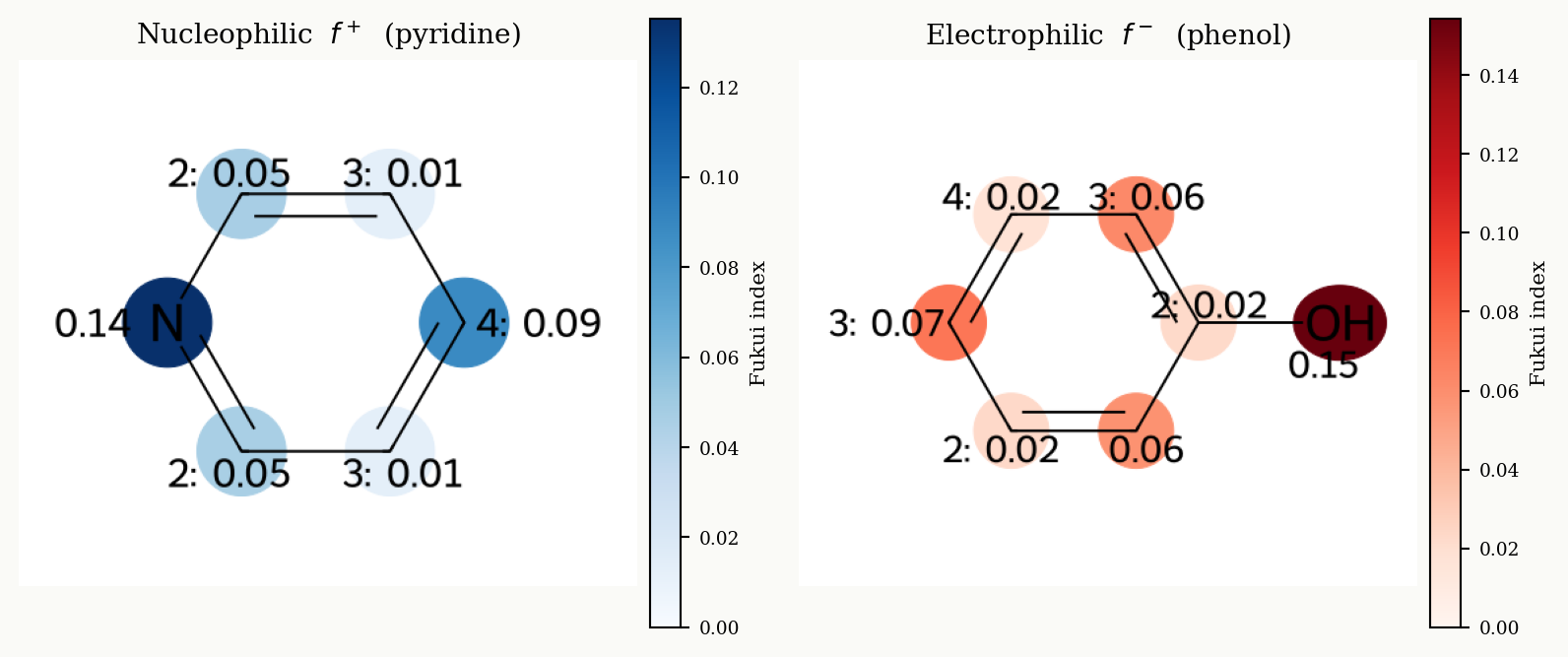
The signs can be counter-intuitive, so it helps to read $f^+$ as *"where does added electron density go?"* — that is the LUMO-like site that an electron-rich **nucleophile** seeks; conversely $f^-$ measures where removing electrons costs the least, the HOMO-like site an **electrophile** attacks. The atom with the **largest** index is the predicted reactive site. Nucleophilic aromatic substitution (S$_N$Ar) is governed by $f^+$ (where a nucleophile adds); electrophilic aromatic substitution (EAS) by $f^-$; and radical C–H functionalization of N-heteroarenes can be ranked by $f^0$ — in published work the highest-$f^0$ atom matches the experimentally observed site of functionalization (e.g. [@ma2014fukui]).
Computing *true* Fukui indices requires three separate single-point calculations — the neutral molecule and its cation and anion at the *same* geometry ($N$, $N{-}1$, $N{+}1$ electrons) — followed by an atomic-population analysis. The figure below carries out exactly that recipe with a small DFT calculation (B3LYP/6-31G). It uses **Mulliken** populations, the simplest version of the original prescription, and maps the resulting **condensed Fukui indices** onto two textbook cases: the nucleophilic index $f^+$ on **pyridine** and the electrophilic index $f^-$ on **phenol**. Mulliken charges are strongly basis-set dependent and are **not recommended for production work**; prefer a real-space partition such as Hirshfeld or CM5.
```{python}
#| label: fig-fukui
#| fig-cap: "Condensed Fukui indices from a small DFT calculation (B3LYP/6-31G, three single points at the neutral geometry). Ring atoms are labelled by their position relative to the heteroatom. Left: among the ring carbons of pyridine the nucleophilic index f+ is largest at the 4- and 2-positions and smallest at the 3-position, matching where nucleophiles add; the nitrogen itself carries the single largest value but is not a substitution site. Right: the electrophilic index f- on phenol is largest on the ortho/para positions, the sites of electrophilic aromatic substitution. The indices do not resolve 2- versus 4- (or ortho versus para): pyridine has two equivalent 2-positions against a single 4-position (phenol, two ortho against one para), a multiplicity the per-atom index does not carry, and the split between them is set mainly by the attacking nucleophile or electrophile. Disc colour and the printed number give the Fukui value at each atom."
import numpy as np
import matplotlib
import matplotlib.pyplot as plt
from io import BytesIO
from PIL import Image
from rdkit import Chem
from rdkit.Chem import AllChem
from rdkit.Chem.Draw import rdMolDraw2D

# SMILES for each panel.
SMILES = {
    "pyridine_fplus": "c1ccncc1",
    "phenol_fminus": "c1ccccc1O",
}

# Condensed Fukui indices, precomputed once with PySCF (B3LYP/6-31G: three
# single points N, N-1, N+1 at the neutral geometry, Mulliken populations) and
# hard-coded here so the chapter renders instantly — no DFT runs at build time.
fukui = {
    "pyridine_fplus": [
        0.08845432741724579,
        0.013564584745770603,
        0.046503549526534016,
        0.13528518184672045,
        0.04650806247914829,
        0.01354911791494473,
    ],
    "phenol_fminus": [
        0.058103906855269116,
        0.023058290909734325,
        0.07169805427696119,
        0.017245078770147693,
        0.06236494418084071,
        0.02289280907021407,
        0.1543379463571597,
    ],
}
# Ring-position labels (2-, 3-, 4- relative to the heteroatom), so it is
# unambiguous which printed value belongs to which position.
POSITIONS = {
    "pyridine_fplus": {2: "2", 4: "2", 1: "3", 5: "3", 0: "4"},
    "phenol_fminus": {1: "2", 5: "2", 2: "3", 4: "3", 3: "4"},
}


def fukui_image(smiles, weights, cmap_name, positions=None):
    mol = Chem.MolFromSmiles(smiles)
    AllChem.Compute2DCoords(mol)
    norm = matplotlib.colors.Normalize(vmin=0, vmax=max(weights))
    cmap = matplotlib.colormaps[cmap_name]
    atom_colors = {i: cmap(norm(w)) for i, w in enumerate(weights)}
    radii = {i: 0.45 for i in range(len(weights))}
    positions = positions or {}
    for i, w in enumerate(weights):
        label = f"{positions[i]}: {w:.2f}" if i in positions else f"{w:.2f}"
        mol.GetAtomWithIdx(i).SetProp("atomNote", label)
    d = rdMolDraw2D.MolDraw2DCairo(470, 400)
    d.drawOptions().annotationFontScale = 0.75
    rdMolDraw2D.PrepareAndDrawMolecule(
        d,
        mol,
        highlightAtoms=list(range(len(weights))),
        highlightAtomColors=atom_colors,
        highlightAtomRadii=radii,
    )
    d.FinishDrawing()
    return Image.open(BytesIO(d.GetDrawingText())), norm, cmap


plt.rcParams.update({"font.family": "serif", "figure.facecolor": "#fafaf7"})
fig, axes = plt.subplots(1, 2, figsize=(8.4, 4.3))
panels = [
    ("pyridine_fplus", "Blues", "Nucleophilic  $f^+$  (pyridine)"),
    ("phenol_fminus", "Reds", "Electrophilic  $f^-$  (phenol)"),
]
for ax, (key, cmap_name, title) in zip(axes, panels):
    img, norm, cmap = fukui_image(SMILES[key], fukui[key], cmap_name, POSITIONS[key])
    ax.imshow(img)
    ax.axis("off")
    ax.set_title(title, fontsize=10.5)
    cb = fig.colorbar(
        matplotlib.cm.ScalarMappable(norm=norm, cmap=cmap),
        ax=ax,
        fraction=0.046,
        pad=0.02,
    )
    cb.set_label("Fukui index", fontsize=8)
    cb.ax.tick_params(labelsize=7)
plt.tight_layout()
plt.show()
```
::: {.callout-note}
These are condensed-to-atom Fukui indices from Mulliken populations at B3LYP/6-31G, evaluated at the fixed neutral geometry (the *vertical* approximation).^[We obtain each index as a difference of **Mulliken** atomic populations between the $N$ and $N\pm1$ species — the original condensed-Fukui prescription of @yang1986fukui. A more rigorous route integrates the Fukui function $f(\mathbf{r})$ over real-space atomic basins (Hirshfeld, or Bader/QTAIM zero-flux basins); for any such real-space partition the population difference *equals* the basin integral, $f_k^\pm = \int_{\Omega_k} f^\pm(\mathbf{r})\,d\mathbf{r}$. Mulliken is instead a basis-set-dependent Hilbert-space partition, so it is the simplest but crudest version and does not correspond to integrating over a spatial basin.] The chemically meaningful part is the *ring-carbon* ordering: $f^+$ peaks on pyridine's 2- and 4-positions — exactly where nucleophiles add (Chichibabin amination, S$_N$Ar) — while $f^-$ peaks on phenol's *ortho*/*para* carbons, the observed sites of electrophilic aromatic substitution. The heteroatoms (N, O) carry the very largest values, since added or removed electron density localizes there, but they are not the C–H substitution sites.
What the indices *cannot* do is choose between the 2- and the 4-position (or, on phenol, between *ortho* and *para*). Two effects are missing. First, multiplicity: pyridine has **two** equivalent 2-positions and only **one** 4-position, and phenol has two *ortho* carbons and a single *para* carbon. Symmetry-equivalent atoms carry identical Fukui values, and the condensed index is a per-atom quantity that says nothing about how many such atoms the molecule has — so even for two sites with exactly equal indices the statistical factor of two already tilts the product ratio toward 2- (or *ortho*). Second, the reagent: which of the two positions wins is largely set by the attacking partner and the conditions, not by the substrate's ground-state electron density. Chichibabin amination with NaNH$_2$ goes cleanly to C2, where the counter-ion can coordinate the ring nitrogen and deliver the nucleophile, whereas bulky nucleophiles are pushed toward the sterically open 4-position; on phenol the *ortho*/*para* ratio tracks the size of the electrophile, with bulky electrophiles (e.g. *tert*-butylation) giving almost exclusively the *para* product. Fukui indices therefore separate reactive sites from unreactive ones — 2-/4- over 3- on pyridine, *ortho*/*para* over *meta* on phenol — but resolving the 2- versus 4- split needs the reaction partner, the solvent, and ultimately the transition state.
Note also that ground-state Fukui indices capture frontier-orbital control well; they do *not* capture cases dominated by intermediate stability, such as the meta-selectivity of nitrobenzene.
:::
## Physics-inspired descriptors
The QM descriptors above are hand-picked scalar quantities. A more systematic goal is to turn raw **3D coordinates** into a single fixed-length vector that an ML model can consume — and to do so by *mimicking how physics computes energy*. The guiding principle is the **many-body expansion**, in which the total energy decomposes into one-body, two-body, three-body, … contributions:
$$
E = V_0 + \sum_i V_1(\mathbf{r}_i) + \sum_{i,j} V_2(r_{ij}) + \sum_{i,j,k} V_3(\theta_{ijk}, \dots) + \cdots
$$
Two-body terms depend on interatomic *distances*, three-body terms on *angles*, and so on, and properties are often built as **sums of atomic contributions** $E = \sum_i E_i$. A good descriptor should encode this same hierarchy.
### Required properties of a good representation
Before building any descriptor, it is worth stating what makes one *good*. A representation should be:
- **Permutation-invariant**: re-labeling identical atoms must not change the vector.
- **Rotation-invariant**: rotating the molecule in space must not change the vector.
- **Translation-invariant**: moving the molecule must not change the vector.
- **Complete**: different structures must map to different vectors (no two distinct geometries collapse to the same point).
- **Smooth**: a small change in geometry produces a small change in the vector (so the learned function is well-behaved).
- **Additive**: the representation should support building a total property as a sum of atomic contributions.
The first three are *symmetries* — physical operations that leave the energy unchanged must leave the descriptor unchanged. The last three control how learnable and expressive the descriptor is. Different descriptors satisfy these to different degrees, and the failures are instructive.
### The Coulomb matrix
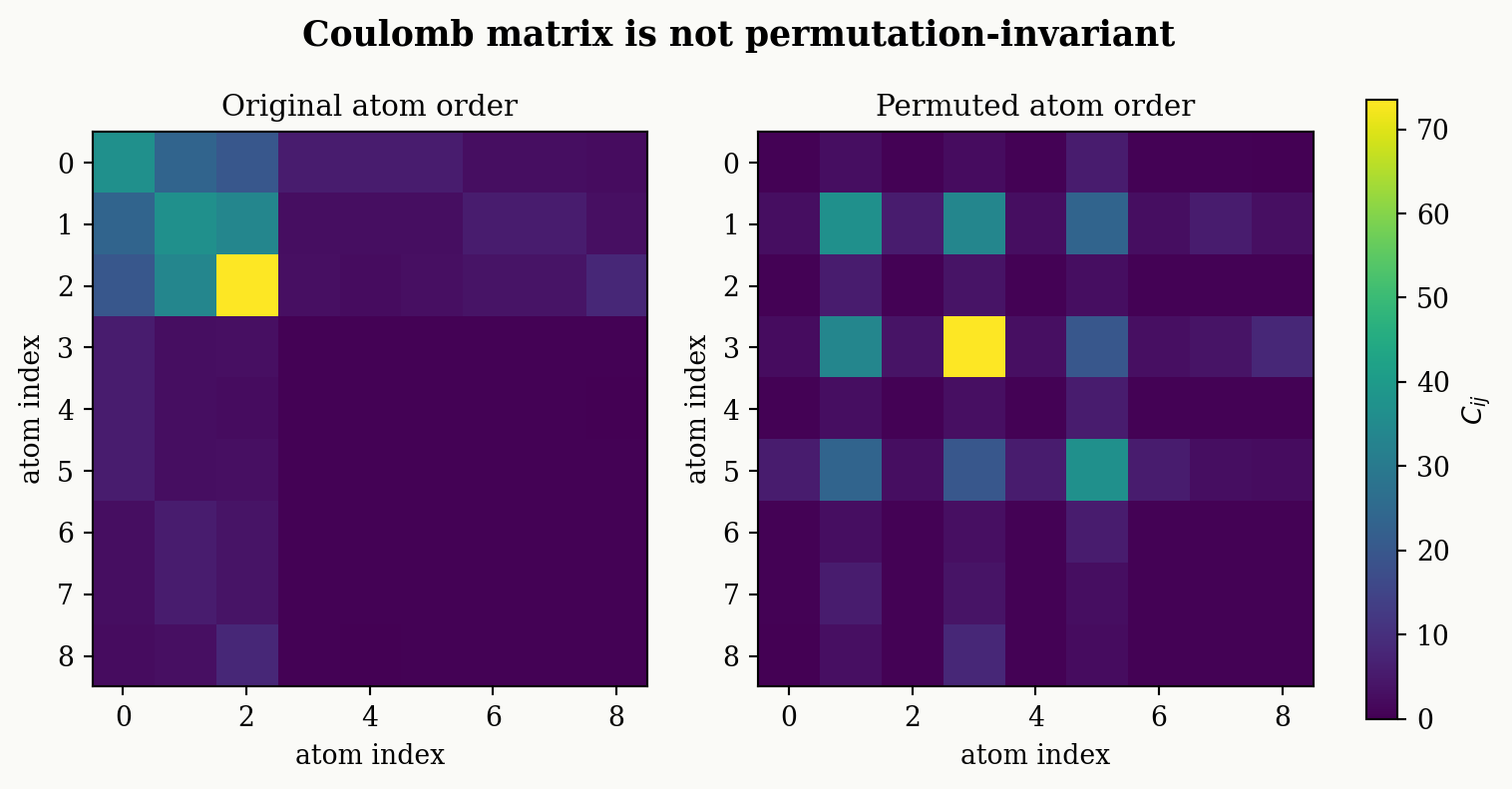
The simplest physics-inspired descriptor is the **Coulomb matrix** [@rupp2012coulomb]. A model needs a vector, not a matrix, so the matrix is **unravelled** into one. Since it is symmetric, only the upper triangle and diagonal are read out, in a fixed order, giving a vector of length $N(N+1)/2$. This is then zero-padded to a common length so molecules of different sizes give vectors of equal size. For a molecule of $N$ atoms the matrix is built from nuclear charges $Z_i$ and interatomic distances $r_{ij}$:
$$
C_{ii} = 0.5\, Z_i^{2.4}, \qquad C_{ij} = \frac{Z_i Z_j}{r_{ij}}.
$$
The diagonal encodes the atoms (a polynomial fit to free-atom energies); the off-diagonal encodes Coulomb-like two-body interactions. Because it depends only on charges and *distances*, the Coulomb matrix is automatically **rotation- and translation-invariant**.
But it is **not permutation-invariant**: if you re-order the atoms, you permute the rows and columns and get a different matrix — even though it is the same molecule. The figure below builds a Coulomb matrix for ethanol from RDKit 3D coordinates and shows that simply shuffling the atom order produces a visibly different matrix.
```{python}
#| label: fig-coulomb-matrix
#| fig-cap: "Coulomb matrix of ethanol (left) and the same molecule with atoms re-ordered (right). The matrices differ, illustrating that the Coulomb matrix is NOT permutation-invariant."
import numpy as np
import matplotlib.pyplot as plt
from rdkit import Chem
from rdkit.Chem import AllChem

plt.rcParams.update({
    "font.family": "serif",
    "figure.facecolor": "#fafaf7",
    "axes.facecolor": "#fafaf7",
})

np.random.seed(2)

# Build 3D ethanol
mol = Chem.AddHs(Chem.MolFromSmiles("CCO"))
AllChem.EmbedMolecule(mol, randomSeed=42)  # ETKDG
AllChem.MMFFOptimizeMolecule(mol)
conf = mol.GetConformer()

Z = np.array([a.GetAtomicNum() for a in mol.GetAtoms()], dtype=float)
coords = np.array([[conf.GetAtomPosition(i).x,
                    conf.GetAtomPosition(i).y,
                    conf.GetAtomPosition(i).z]
                   for i in range(mol.GetNumAtoms())])

def coulomb_matrix(Z, coords):
    n = len(Z)
    C = np.zeros((n, n))
    for i in range(n):
        for j in range(n):
            if i == j:
                C[i, j] = 0.5 * Z[i] ** 2.4
            else:
                r = np.linalg.norm(coords[i] - coords[j])
                C[i, j] = Z[i] * Z[j] / r
    return C

C = coulomb_matrix(Z, coords)

# Permute atom order
perm = np.random.permutation(len(Z))
C_perm = coulomb_matrix(Z[perm], coords[perm])

fig, axes = plt.subplots(1, 2, figsize=(9, 4.2))
vmax = C.max()
for ax, M, title in [(axes[0], C, "Original atom order"),
                     (axes[1], C_perm, "Permuted atom order")]:
    im = ax.imshow(M, cmap="viridis", vmin=0, vmax=vmax)
    ax.set_title(title, fontsize=11)
    ax.set_xlabel("atom index")
    ax.set_ylabel("atom index")
fig.colorbar(im, ax=axes, fraction=0.046, pad=0.04, label=r"$C_{ij}$")
fig.suptitle("Coulomb matrix is not permutation-invariant", fontsize=13, fontweight="bold")
plt.show()
```
The usual fixes restore permutation invariance exactly: **sort** the rows by norm (canonicalization), use the **eigenvalue spectrum** of the matrix (invariant to permutation by construction), or decompose into **Bag of Bonds** (group entries by atom-pair type). The invariance they achieve is exact, but some information is lost in this transformation: different environments can map to the same sorted or spectral representation, and, for sorting, smoothness is lost, since a small change in geometry can swap two rows.
### SOAP: Smooth Overlap of Atomic Positions
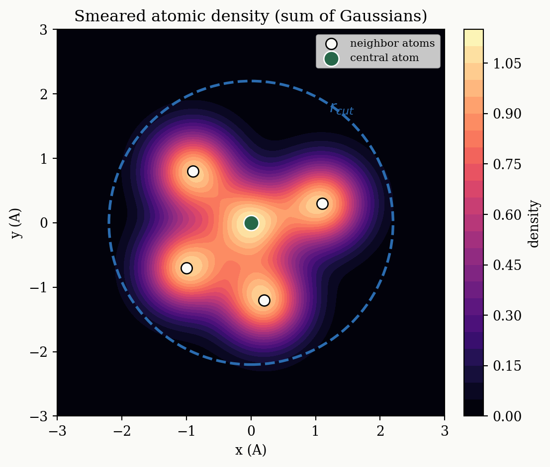
A more powerful and widely used descriptor is **SOAP** (Smooth Overlap of Atomic Positions; [@deringer2021gpr]). Its construction is a direct implementation of the "smear out the atoms and characterize the local density" idea:
1. Place a **Gaussian** on every atom.
2. Sum them to build a smooth **atomic density** $\rho_i(\mathbf{r})$ within a cutoff radius $r_{\text{cut}}$ around a central atom $i$.
3. Expand that density in a basis of **radial** functions and **spherical harmonics** (the angular part).
4. Form the **rotationally averaged power spectrum** — combining the expansion coefficients so that the result is invariant to rotation. That power spectrum *is* the SOAP vector.
The power spectrum correlates the density with itself at two points in space around the central atom. Together with the central atom that makes SOAP a **3-body** descriptor, but note that only the central atom is an atom: the other two are points at which the neighbour density is evaluated, and the neighbours enter only through the density they build up. and it is permutation-, rotation-, and translation-invariant and smooth by construction. The figure below illustrates step 2 — the "smeared" atomic density that SOAP characterizes — by summing 2D Gaussians placed at a few atom positions.
```{python}
#| label: fig-soap-density
#| fig-cap: "The smooth 'smeared' atomic density that SOAP characterizes: a sum of Gaussians placed on atom positions within a cutoff. SOAP expands this density in radial and angular basis functions."
import numpy as np
import matplotlib.pyplot as plt

plt.rcParams.update({
    "font.family": "serif",
    "figure.facecolor": "#fafaf7",
    "axes.facecolor": "#fafaf7",
})

np.random.seed(3)
# A central atom + a few neighbors (toy 2D positions, Angstrom-like)
central = np.array([0.0, 0.0])
neighbors = np.array([
    [1.1, 0.3],
    [-0.9, 0.8],
    [0.2, -1.2],
    [-1.0, -0.7],
])
atoms = np.vstack([central, neighbors])
sigma = 0.45
r_cut = 2.2

# Grid
g = np.linspace(-3, 3, 300)
X, Y = np.meshgrid(g, g)
density = np.zeros_like(X)
for (ax_, ay_) in atoms:
    density += np.exp(-((X - ax_) ** 2 + (Y - ay_) ** 2) / (2 * sigma ** 2))

fig, ax = plt.subplots(figsize=(6, 5))
im = ax.contourf(X, Y, density, levels=25, cmap="magma")
# Cutoff circle around central atom
circle = plt.Circle(central, r_cut, fill=False, color="#2b6cb0", lw=2, ls="--")
ax.add_patch(circle)
ax.scatter(neighbors[:, 0], neighbors[:, 1], color="#fafaf7", edgecolors="black",
           s=70, zorder=5, label="neighbor atoms")
ax.scatter(*central, color="#276749", edgecolors="white", s=130, zorder=6,
           label="central atom")
ax.text(r_cut * 0.55, r_cut * 0.78, r"$r_{cut}$", color="#2b6cb0", fontsize=12)

ax.set_aspect("equal")
ax.set_xlabel("x (A)")
ax.set_ylabel("y (A)")
ax.set_title("Smeared atomic density (sum of Gaussians)")
ax.legend(fontsize=8, loc="upper right")
fig.colorbar(im, ax=ax, fraction=0.046, pad=0.04, label="density")
plt.tight_layout()
plt.show()
```
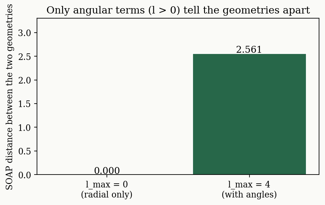
The resolution of SOAP is controlled by a few parameters. The number of radial functions $n_{\max}$ and the maximum angular momentum $l_{\max}$ trade cost for detail, and the cutoff $r_{\text{cut}}$ sets how *local* the environment is. The role of $l_{\max}$ is especially instructive: with **$l_{\max}=0$ you keep only radial (2-body) information** and are completely blind to angles.
We can test this directly. Below we build two geometries with **identical C–H bond lengths** — tetrahedral CH$_4$ and a flattened (pyramidal) version with different H–C–H angles — and compute the SOAP vector at the carbon with `dscribe`, once with $l_{\max}=0$ and once with $l_{\max}=4$.
```{python}
#| label: fig-soap-lmax
#| fig-cap: "SOAP discrimination test. With l_max=0 (radial/2-body only) two geometries with equal bond lengths but different angles give an identical descriptor (distance 0). Adding angular terms (l_max=4) resolves them."
import numpy as np
import matplotlib.pyplot as plt
from ase import Atoms
from dscribe.descriptors import SOAP

d = 1.09  # C-H bond length (Angstrom), identical in both geometries

# Tetrahedral CH4
tet = np.array([[0, 0, 0], [1, 1, 1], [1, -1, -1], [-1, 1, -1], [-1, -1, 1]], float)
tet[1:] = tet[1:] / np.linalg.norm(tet[1:], axis=1, keepdims=True) * d
ch4 = Atoms("CH4", positions=tet)

# Flattened geometry: same bond lengths, different angles
pyr = tet.copy()
pyr[1:, 2] *= 0.5
pyr[1:] = pyr[1:] / np.linalg.norm(pyr[1:], axis=1, keepdims=True) * d
flat = Atoms("CH4", positions=pyr)

dists = []
for lmax in (0, 4):
    soap = SOAP(species=["H", "C"], r_cut=5.0, n_max=4, l_max=lmax, periodic=False)
    v_tet = soap.create(ch4, centers=[0])[0]
    v_flat = soap.create(flat, centers=[0])[0]
    dists.append(np.linalg.norm(v_tet - v_flat))
    print(f"l_max={lmax}: SOAP length={len(v_tet):3d}, "
          f"||tetrahedral - flattened|| = {dists[-1]:.6f}")

fig, ax = plt.subplots(figsize=(5.5, 3.5))
bars = ax.bar(["l_max = 0\n(radial only)", "l_max = 4\n(with angles)"], dists,
              color=["#c53030", "#276749"], edgecolor="white")
ax.set_ylabel("SOAP distance between the two geometries")
ax.set_title("Only angular terms (l > 0) tell the geometries apart")
for b, dval in zip(bars, dists):
    ax.text(b.get_x() + b.get_width()/2, b.get_height() + 0.02,
            f"{dval:.3f}", ha="center", fontsize=11)
ax.set_ylim(0, max(dists) * 1.25 + 0.1)
plt.tight_layout()
plt.show()
```
With $l_{\max}=0$ the two distinct geometries collapse to **exactly the same vector** (distance $0$); only when angular terms are switched on ($l_{\max}=4$) does SOAP tell them apart. This is precisely why a good representation must capture body-orders beyond 2.
### Where these descriptors go
These physics-based descriptors are designed to feed **classical ML** models — in particular kernel methods such as [kernel ridge regression](07_non_linear_models.qmd#kernel-ridge-regression) and [Gaussian process regression](13_optimization.qmd#gaussian-process-regression-gpr), where the descriptor enters a similarity kernel comparing two atomic environments. The same atom-centered, sum-over-atoms philosophy underlies modern **machine-learning interatomic potentials** (ANI, MACE), which learn $E_i$ for each atom and sum to the total energy. Those learned representations — and the [graph neural networks](08_graph_models.qmd) that generalize them — are the subject of a later chapter.
## Summary
- **PES & the cost–accuracy hierarchy.** Chemistry is encoded in the potential energy surface (energy vs. $3N$ coordinates): minima are structures, saddle points are transition states. Computing the energy means approximating the Schrödinger equation, which is intractable exactly. Methods form a hierarchy — force fields → ML potentials → semi-empirical → DFT → correlated wavefunction — and **computational scaling** (from $\sim N$ for force fields up to $M^7$ for CCSD(T)) is the core cost driver, so accuracy gets steeply more expensive.
- **DFT, Jacob's ladder & error cancellation.** DFT works with the electron density; its unknown exchange–correlation functional is approximated, and the approximations climb **Jacob's ladder** (LDA → GGA → meta-GGA → hybrid → double-hybrid). No one knows the exact functional, so test for your use case. **Absolute energies are hard; relative energies are easy** thanks to systematic **error cancellation**. - **DFT, Jacob's ladder & error cancellation.** DFT works with the electron density; its unknown exchange–correlation functional is approximated, and the approximations climb **Jacob's ladder** (LDA → GGA → meta-GGA → hybrid → double-hybrid). No one knows the exact functional, so test for your use case. **Absolute energies are hard; relative energies are more accessible** thanks to systematic **error cancellation** — but only when the species compared are genuinely similar. Distinguish this from mere **trend preservation**, where a large constant offset leaves the ranking of a series intact without anything having cancelled.
- **Semi-empirical ≈ simple ML.** Expensive two-electron integrals are replaced by a few fitted parameters (Pariser–Parr, $\gamma_{\text{AA}} = \text{IP}_{\text{A}} - \text{EA}_{\text{A}}$; AM1, PM6, GFN2-xTB), making these methods the conceptual bridge from physics to ML.
- **QM descriptors & Fukui.** Computed quantum quantities (charges, HOMO/LUMO, **Fukui indices** $f^+, f^-, f^0$) serve as electronic-structure-rich input features; the largest Fukui index predicts the reactive site.
- **Physics-based descriptors.** Turn 3D coordinates into a vector via the many-body expansion. A good representation is invariant to **permutation, rotation, and translation**, plus complete, smooth, and additive. The **Coulomb matrix** is rotation/translation-invariant but not permutation-invariant (fix by sorting, eigenvalues, or Bag of Bonds); **SOAP** smears atoms into a density and builds a rotationally averaged 3-body power spectrum, needing $l_{\max}>0$ to capture angles.